Python Machine Learning Tutorial

Machine Learning

---

What is TensorFlow

The official TensoFlow website tensorflow.org writes: "TensorFlow™ is an open source software library for high performance numerical computation. Its flexible architecture allows easy deployment of computation across a variety of platforms (CPUs, GPUs, TPUs), and from desktops to clusters of servers to mobile and edge devices. Originally developed by researchers and engineers from the Google Brain team within Google’s AI organization, it comes with strong support for machine learning and deep learning and the flexible numerical computation core is used across many other scientific domains."

---

This website is created by:



Python Training Courses

---

Follow Bernd Klein, the author of this website, at Google+:
Bernd Klein on Google

Bernd Klein on Facebook


Search this website:

Classroom Training Courses

This website contains a free and extensive online tutorial by Bernd Klein, using material from his classroom Python training courses.

If you are interested in an instructor-led classroom training course, you may have a look at the Python classes
by Bernd Klein at Bodenseo. © kabliczech - Fotolia.com

Quote of the Day:

"The internet could be a very positive step towards education, organisation and participation in a meaningful society." (Noam Chomsky)

---

If you have the choice working with Python 2 or Python 3, we recomend to switch to Python 3! You can read our Python Tutorial to see what the differences are.

Data Protection Declaration

Data Protection Declaration

TensorFlow

TensorFlow is an open-sourse software library for machine learning across a range of tasks. It is a symbolic math library, and also used as a system for building and training neural networks to detect and decipher patterns and correlations, analogous to human learning and reasoning. It is used for both research and production at Google often replacing its closed-source predecessor, DistBelief. TensorFlow was developed by the Google Brain team for internal Google use. It was released under the Apache 2.0 open source license on 9 November 2015.

TensorFlow provides a Python API as well as C++, Haskell, Java, Go and Rust APIs.

A tensor can be represented as a multidimensional array of numbers. A tensor has its rank and shape, rank is its number of dimensions and shape is the size of each dimension.

# a rank 0 tensor, i.e. a scalar with shape ():
42                     
# a rank 1 tensor, i.e. a vector with shape (3,):
[1, 2, 3] 
# a rank 2 tensor, i.e. a matrix with shape (2, 3):           
[[1, 2, 3], [3, 2, 1]] 
# a rank 3 tensor with shape (2, 2, 2) :
[ [[3, 4], [1, 2]], [[3, 5], [8, 9]]] 
#

The previous Python code returned the following result:

[[[3, 4], [1, 2]], [[3, 5], [8, 9]]]

All data of TensorFlow is represented as tensors. It is the sole data structure:

tf.float32, tf.float64, tf.int8, tf.int16, …, tf.int64, tf.uint8, ...

Structure of TensorFlow Programs

TensorFlow programs consist of two discrete sections:

1. A graph is created in the construction phase.
2. The computational graph is run in the execution phase, which is a session.

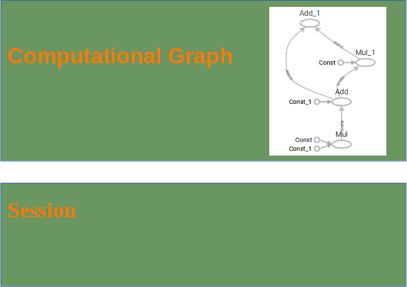
Example

import tensorflow as tf
# Computational Graph:
c1 = tf.constant(0.034)
c2 = tf.constant(1000.0)
x = tf.multiply(c1, c1)
y = tf.multiply(c1, c2)
final_node = tf.add(x, y)
# Running the session:
with tf.Session() as sess:
    result = sess.run(final_node)
    print(result, type(result))

34.0012 <class 'numpy.float32'>

import tensorflow as tf
# Computational Graph:
c1 = tf.constant(0.034, dtype=tf.float64)
c2 = tf.constant(1000.0, dtype=tf.float64)
x = tf.multiply(c1, c1)
y = tf.multiply(c1, c2)
final_node = tf.add(x, y)
# Running the session:
with tf.Session() as sess:
    result = sess.run(final_node)
    print(result, type(result))

34.001156 <class 'numpy.float64'>

import tensorflow as tf
# Computational Graph:
c1 = tf.constant([3.4, 9.1, -1.2, 9], dtype=tf.float64)
c2 = tf.constant([3.4, 9.1, -1.2, 9], dtype=tf.float64)
x = tf.multiply(c1, c1)
y = tf.multiply(c1, c2)
final_node = tf.add(x, y)
# Running the session:
with tf.Session() as sess:
    result = sess.run(final_node)
    print(result, type(result))

[  23.12  165.62    2.88  162.  ] <class 'numpy.ndarray'>

A computational graph is a series of TensorFlow operations arranged into a graph of nodes. Let's build a simple computational graph. Each node takes zero or more tensors as inputs and produces a tensor as an output. Constant nodes take no input.

Printing the nodes does not output a numerical value. We have defined a computational graph but no numerical evaluation has taken place!

c1 = tf.constant([3.4, 9.1, -1.2, 9], dtype=tf.float64)
c2 = tf.constant([3.4, 9.1, -1.2, 9], dtype=tf.float64)
x = tf.multiply(c1, c1)
y = tf.multiply(c1, c2)
final_node = tf.add(x, y)
print(c1)
print(x)
print(final_node)

Tensor("Const_6:0", shape=(4,), dtype=float64)
Tensor("Mul_6:0", shape=(4,), dtype=float64)
Tensor("Add_3:0", shape=(4,), dtype=float64)

To evaluate the nodes, we have to run the computational graph within a session. A session encapsulates the control and state of the TensorFlow runtime. The following code creates a Session object and then invokes its run method to run enough of the computational graph to evaluate node1 and node2. By running the computational graph in a session as follows. We have to create a session object:

session = tf.Session()

Now, we can evaluate the computational graph by starting the run method of the session object:

result = session.run(final_node)
print(result)
print(type(result))

[  23.12  165.62    2.88  162.  ]
<class 'numpy.ndarray'>

Of course, we will have to close the session, when we are finished:

session.close()

It is usually a better idea to work with the with statement, as we did in the introductory examples!

Similarity to NumPy

We will rewrite the following program with Numpy.

import tensorflow as tf
session = tf.Session()
x = tf.range(12)
print(session.run(x))
x2 = tf.reshape(tensor=x, 
                shape=(3, 4))
x2 = tf.reduce_sum(x2, reduction_indices=[0])
res = session.run(x2)
print(res)
x3 = tf.eye(5, 5)
res = session.run(x3)
print(res)

[ 0  1  2  3  4  5  6  7  8  9 10 11]
[12 15 18 21]
[[ 1.  0.  0.  0.  0.]
 [ 0.  1.  0.  0.  0.]
 [ 0.  0.  1.  0.  0.]
 [ 0.  0.  0.  1.  0.]
 [ 0.  0.  0.  0.  1.]]

Now a similar Numpy version:

import numpy as np
x = np.arange(12)
print(x)
x2 = x.reshape((3, 4))
res = x2.sum(axis=0)
print(res)
x3 = np.eye(5, 5)
print(x3)

[ 0  1  2  3  4  5  6  7  8  9 10 11]
[12 15 18 21]
[[ 1.  0.  0.  0.  0.]
 [ 0.  1.  0.  0.  0.]
 [ 0.  0.  1.  0.  0.]
 [ 0.  0.  0.  1.  0.]
 [ 0.  0.  0.  0.  1.]]

TensorBoard

• TensorFlow provides functions to debug and optimize programs with the help of a visualization tool called TensorBoard.
• TensorFlow creates the necessary data during its execution.
• The data are stored in trace files.
• Tensorboard can be viewed from a browser using http://localhost:6006/

We can run the following example program, and it will create the directory "output" We can run now tensorboard: tensorboard --logdir output

which will create a webserver: TensorBoard 0.1.8 at http://marvin:6006 (Press CTRL+C to quit)

import tensorflow as tf
p = tf.constant(0.034)
c = tf.constant(1000.0)
x = tf.add(c, tf.multiply(p, c))
x = tf.add(x, tf.multiply(p, x))
with tf.Session() as sess:
    writer = tf.summary.FileWriter("output", sess.graph)
    print(sess.run(x))
    writer.close()

1069.16

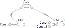
The computational graph is included in the TensorBoard:

Placeholders

A computational graph can be parameterized to accept external inputs, known as placeholders. The values for placeholders are provided when the graph is run in a session.

import tensorflow as tf
c1 = tf.placeholder(tf.float32)
c2 = tf.placeholder(tf.float32)
x = tf.multiply(c1, c1)
y = tf.multiply(c1, c2)
final_node = tf.add(x, y)
with tf.Session() as sess:
    result = final_node.eval( {c1: 3.8, c2: 47.11})
    print(result)
    result = final_node.eval( {c1: [3, 5], c2: [1, 3]})
    print(result)

193.458
[ 12.  40.]

Another example:

import tensorflow  as tf
import numpy as np
v1 = np.array([3, 4, 5])
v2 = np.array([4, 1, 1])
c1 = tf.placeholder(tf.float32, shape=(3,))
c2 = tf.placeholder(tf.float32, shape=(3,))
x = tf.multiply(c1, c1)
y = tf.multiply(c1, c2)
final_node = tf.add(x, y)
with tf.Session() as sess:
    result = final_node.eval( {c1: v1, c2: v2})
    print(result)

[ 21.  20.  30.]

placeholder( dtype, shape=None, name=None )

Inserts a placeholder for a tensor that will be always fed. It returns a Tensor that may be used as a handle for feeding a value, but not evaluated directly.

Important: This tensor will produce an error if evaluated. Its value must be fed using the feed_dict optional argument to

Session.run()

Tensor.eval()

Operation.run()

Args:

Parameter	Description
dtype:	The type of elements in the tensor to be fed.
shape:	The shape of the tensor to be fed (optional). If the shape is not specified, you can feed a tensor of any shape.
name:	A name for the operation (optional).

Variables

Variables are used to add trainable parameters to a graph. They are constructed with a type and initial value. Variables are not initialized when you call tf.Variable. To initialize the variables of a TensorFlow graph, we have to call global_variables_initializer:

import tensorflow as tf
W = tf.Variable([.5], dtype=tf.float32)
b = tf.Variable([-1], dtype=tf.float32)
x = tf.placeholder(tf.float32)
model = W * x + b
with tf.Session() as sess:
    init = tf.global_variables_initializer()
    sess.run(init)
    print(sess.run(model, {x: [1, 2, 3, 4]}))

[-0.5  0.   0.5  1. ]

Difference Between Variables and Placeholders

The difference between tf.Variable and tf.placeholder consists in the time when the values are passed. If you use tf.Variable, you have to provide an initial value when you declare it. With tf.placeholder you don't have to provide an initial value.

The value can be specified at run time with the feed_dict argument inside Session.run

A placeholder is used for feeding external data into a Tensorflow computation, i.e. from outside of the graph!

If you are training a learning algorithm, a placeholder is used for feeding in your training data. This means that the training data is not part of the computational graph. The placeholder behaves similar to the Python "input" statement. On the other hand a TensorFlow variable behaves more or less like a Python variable!

Example:

Calculating the loss:

import tensorflow as tf
W = tf.Variable([.5], dtype=tf.float32)
b = tf.Variable([-1], dtype=tf.float32)
x = tf.placeholder(tf.float32)
y = tf.placeholder(tf.float32)
model = W * x + b
deltas = tf.square(model - y)
loss = tf.reduce_sum(deltas)
with tf.Session() as sess:
    init = tf.global_variables_initializer()
    sess.run(init)
 
    print(sess.run(loss, {x: [1, 2, 3, 4], y: [1, 1, 1, 1]}))

3.5

Reassigning Values to Variables

import tensorflow as tf
W = tf.Variable([.5], dtype=tf.float32)
b = tf.Variable([-1], dtype=tf.float32)
x = tf.placeholder(tf.float32)
y = tf.placeholder(tf.float32)
model = W * x + b
deltas = tf.square(model - y)
loss = tf.reduce_sum(deltas)
with tf.Session() as sess:
    init = tf.global_variables_initializer()
    sess.run(init)
 
    print(sess.run(loss, {x: [1, 2, 3, 4], y: [1, 1, 1, 1]}))
    W_a = tf.assign(W, [0.])
    b_a =  tf.assign(b, [1.])
    sess.run( W_a )
    sess.run( b_a)  
    # sess.run( [W_a, b_a] ) # alternatively in one 'run'
   
    print(sess.run(loss, {x: [1, 2, 3, 4], y: [1, 1, 1, 1]}))

3.5
0.0

import tensorflow as tf
W = tf.Variable([.5], dtype=tf.float32)
b = tf.Variable([-1], dtype=tf.float32)
x = tf.placeholder(tf.float32)
y = tf.placeholder(tf.float32)
model = W * x + b
deltas = tf.square(model - y)
loss = tf.reduce_sum(deltas)
optimizer = tf.train.GradientDescentOptimizer(0.01)
train = optimizer.minimize(loss)
with tf.Session() as sess:
    init = tf.global_variables_initializer()
    sess.run(init)
    for _ in range(1000):
        sess.run(train, 
                  {x: [1, 2, 3, 4], y: [1, 1, 1, 1]})
    writer = tf.summary.FileWriter("optimizer", sess.graph)
    print(sess.run([W, b]))
    writer.close()

[array([  3.91378126e-06], dtype=float32), array([ 0.99998844], dtype=float32)]

Creating Data Sets

We will create data sets for a larger example for the GradientDescentOptimizer.

import numpy as np
import matplotlib.pyplot as plt
for quantity, suffix in [(1000, "train"), (200, "test")]:
    samples = np.random.multivariate_normal([-2, -2], [[1, 0], [0, 1]], quantity)
    plt.plot(samples[:, 0], samples[:, 1], '.', label="bad ones " + suffix)
    bad_ones = np.column_stack((np.zeros(quantity), samples))
    
    samples = np.random.multivariate_normal([1, 1], [[1, 0.5], [0.5, 1]], quantity)
    plt.plot(samples[:, 0], samples[:, 1], '.', label="good ones " + suffix)
    good_ones = np.column_stack((np.ones(quantity), samples))
    
    sample = np.row_stack((bad_ones, good_ones))
    np.savetxt("data/the_good_and_the_bad_ones_" + suffix + ".txt", sample, fmt="%1d %4.2f %4.2f")
    
plt.legend()
plt.show()

import os
os.environ['TF_CPP_MIN_LOG_LEVEL']='2'
import numpy as np
import tensorflow as tf
from matplotlib import pyplot as plt
number_of_samples_per_training_step = 100
num_of_epochs = 1  
num_labels = 2 # should be automatically determined
def evaluation_func(X):
    return predicted_class.eval(feed_dict={x:X}) 
def plot_boundary(X, Y, pred_func):
    # determine canvas borders
    mins = np.amin(X, 0)    # array with column minimums
    mins = mins - 0.1*np.abs(mins)
    maxs = np.amax(X, 0)    # array with column maximums
    maxs = maxs + 0.1*maxs
    xs, ys = np.meshgrid(np.linspace(mins[0], maxs[0], 300), 
                         np.linspace(mins[1], maxs[1], 300))
    # evaluate model using the dense grid
    # c_ creates one array with "points" from meshgrid:
    
    Z = pred_func(np.c_[xs.flatten(), ys.flatten()])
    # Z is one-dimensional and will be reshaped into 300 x 300:  
    Z = Z.reshape(xs.shape) 
    
    # Plot the contour and training examples
    plt.contourf(xs, ys, Z, colors=('c', 'g', 'y', 'b'))
    Xn = X[Y[:,1]==1]
    plt.plot(Xn[:, 0], Xn[:, 1], "bo")
    Xn = X[Y[:,1]==0]
    plt.plot(Xn[:, 0], Xn[:, 1], "go")
    plt.show()
def get_data(fname):
    data = np.loadtxt(fname)
    labels = data[:, :1] #  array([[ 0.], [ 0.], [ 1.], ...]])
    labels_one_hot = (np.arange(num_labels) == labels).astype(np.float32)
    data = data[:, 1:].astype(np.float32)
    return data, labels_one_hot
data_train = "data/the_good_and_the_bad_ones_train.txt"
data_test = "data/the_good_and_the_bad_ones_test.txt"
train_data, train_labels = get_data(data_train)
test_data, test_labels = get_data(data_test)
train_size, num_features = train_data.shape
x = tf.placeholder("float", shape=[None, num_features])
y_ = tf.placeholder("float", shape=[None, num_labels])
   
Weights = tf.Variable(tf.zeros([num_features, num_labels]))
b = tf.Variable(tf.zeros([num_labels]))
y = tf.nn.softmax(tf.matmul(x, Weights) + b)
# Optimization.
cross_entropy = -tf.reduce_sum(y_*tf.log(y))
train_step = tf.train.GradientDescentOptimizer(0.01).minimize(cross_entropy)
# For the test data, hold the entire dataset in one constant node.
test_data_node = tf.constant(test_data)
# Evaluation.
predicted_class = tf.argmax(y, 1)
correct_prediction = tf.equal(tf.argmax(y,1), tf.argmax(y_,1))
accuracy = tf.reduce_mean(tf.cast(correct_prediction, "float"))
with tf.Session() as sess:
    # Run all the initializers to prepare the trainable parameters.
    init = tf.global_variables_initializer()
    
    sess.run(init)
        
    # Iterate and train.
    for step in range(num_of_epochs * train_size // number_of_samples_per_training_step):
    
        offset = (step * number_of_samples_per_training_step) % train_size
        # get a batch of data
        batch_data = train_data[offset:(offset + 
                                        number_of_samples_per_training_step), :]
        batch_labels = train_labels[offset:(offset + number_of_samples_per_training_step)]
        
        # feed data into the model
        train_step.run(feed_dict={x: batch_data, y_: batch_labels})
    print('\nBias vector: ', sess.run(b))
    print('Weight matrix:\n', sess.run(Weights))
    print("\nApplying model to first data set:")
    first = test_data[:1]
    print(first)
    print("\nWx + b: ", sess.run(tf.matmul(first, Weights) + b))
    # the softmax function, or normalized exponential function, is a generalization of the 
    # logistic function that "squashes" a K-dimensional vector z of arbitrary real values 
    # to a K-dimensional vector σ(z) of real values in the range [0, 1] that add up to 1. 
    print("softmax(Wx + b): ", sess.run(tf.nn.softmax(tf.matmul(first, Weights) + b)))
    print("Accuracy on test data: ", accuracy.eval(feed_dict={x: test_data, y_: test_labels}))
    print("Accuracy on training data: ", accuracy.eval(feed_dict={x: train_data, y_: train_labels}))
    
    # classify some values:
    print(evaluation_func([[-3, 7.3], [-1,8], [0, 0], [1, 0.0], [-1, 0]]))    
        
    plot_boundary(test_data, test_labels, evaluation_func)
    

The above code returned the following:

Bias vector:  [-0.78089082  0.78089082]
Weight matrix:
 [[-0.80193734  0.8019374 ]
 [-0.831303    0.831303  ]]
Applying model to first data set:
[[-1.05999994 -1.55999994]]
Wx + b:  [[ 1.36599553 -1.36599553]]
softmax(Wx + b):  [[ 0.93888813  0.06111182]]
Accuracy on test data:  0.97
Accuracy on training data:  0.9725
[1 1 1 1 0]

© 2011 - 2018, Bernd Klein, Bodenseo; Design by Denise Mitchinson adapted for python-course.eu by Bernd Klein