2. Creating Numpy Arrays
By Bernd Klein. Last modified: 24 Mar 2022.

We have alreday seen in the previous chapter of our Numpy tutorial that we can create Numpy arrays from lists and tuples. We want to introduce now further functions for creating basic arrays.
There are functions provided by Numpy to create arrays with evenly spaced values within a given interval. One 'arange' uses a given distance and the other one 'linspace' needs the number of elements and creates the distance automatically.
Creation of Arrays with Evenly Spaced Values
arange
The syntax of arange:
arange([start,] stop[, step], [, dtype=None])
arange returns evenly spaced values within a given interval. The values are generated within the half-open interval '[start, stop)' If the function is used with integers, it is nearly equivalent to the Python built-in function range, but arange returns an ndarray rather than a list iterator as range does. If the 'start' parameter is not given, it will be set to 0. The end of the interval is determined by the parameter 'stop'. Usually, the interval will not include this value, except in some cases where 'step' is not an integer and floating point round-off affects the length of output ndarray. The spacing between two adjacent values of the output array is set with the optional parameter 'step'. The default value for 'step' is 1. If the parameter 'step' is given, the 'start' parameter cannot be optional, i.e. it has to be given as well. The type of the output array can be specified with the parameter 'dtype'. If it is not given, the type will be automatically inferred from the other input arguments.
import numpy as np

a = np.arange(1, 10)
print(a)

x = range(1, 10)
print(x)    # x is an iterator
print(list(x))

# further arange examples:
x = np.arange(10.4)
print(x)
x = np.arange(0.5, 10.4, 0.8)
print(x)
OUTPUT:
[1 2 3 4 5 6 7 8 9]
range(1, 10)
[1, 2, 3, 4, 5, 6, 7, 8, 9]
[ 0.  1.  2.  3.  4.  5.  6.  7.  8.  9. 10.]
[ 0.5  1.3  2.1  2.9  3.7  4.5  5.3  6.1  6.9  7.7  8.5  9.3 10.1]
Be careful, if you use a float value for the step parameter, as you can see in the following example:
np.arange(12.04, 12.84, 0.08)
OUTPUT:
array([12.04, 12.12, 12.2 , 12.28, 12.36, 12.44, 12.52, 12.6 , 12.68,
       12.76, 12.84])
The help of arange has to say the following for the stop parameter: "End of interval. The interval does not include this value, except in some cases where step is not an integer and floating point round-off affects the length of out. This is what happened in our example.
The following usages of arange is a bit offbeat. Why should we use float values, if we want integers as result. Anyway, the result might be confusing. Before arange starts, it will round the start value, end value and the stepsize:
x = np.arange(0.5, 10.4, 0.8, int)
print(x)
OUTPUT:
[ 0 1 2 3 4 5 6 7 8 9 10 11 12]
This result defies all logical explanations. A look at help also helps here: "When using a non-integer step, such as 0.1, the results will often not be consistent. It is better to use numpy.linspace for these cases. Using linspace is not an easy workaround in some situations, because the number of values has to be known.
linspace
The syntax of linspace:
linspace(start, stop, num=50, endpoint=True, retstep=False)
linspace returns an ndarray, consisting of 'num' equally spaced samples in the closed interval [start, stop] or the half-open interval [start, stop). If a closed or a half-open interval will be returned, depends on whether 'endpoint' is True or False. The parameter 'start' defines the start value of the sequence which will be created. 'stop' will the end value of the sequence, unless 'endpoint' is set to False. In the latter case, the resulting sequence will consist of all but the last of 'num + 1' evenly spaced samples. This means that 'stop' is excluded. Note that the step size changes when 'endpoint' is False. The number of samples to be generated can be set with 'num', which defaults to 50. If the optional parameter 'endpoint' is set to True (the default), 'stop' will be the last sample of the sequence. Otherwise, it is not included.
import numpy as np

# 50 values between 1 and 10:
print(np.linspace(1, 10))
# 7 values between 1 and 10:
print(np.linspace(1, 10, 7))
# excluding the endpoint:
print(np.linspace(1, 10, 7, endpoint=False))
OUTPUT:
[ 1.          1.18367347  1.36734694  1.55102041  1.73469388  1.91836735
  2.10204082  2.28571429  2.46938776  2.65306122  2.83673469  3.02040816
  3.20408163  3.3877551   3.57142857  3.75510204  3.93877551  4.12244898
  4.30612245  4.48979592  4.67346939  4.85714286  5.04081633  5.2244898
  5.40816327  5.59183673  5.7755102   5.95918367  6.14285714  6.32653061
  6.51020408  6.69387755  6.87755102  7.06122449  7.24489796  7.42857143
  7.6122449   7.79591837  7.97959184  8.16326531  8.34693878  8.53061224
  8.71428571  8.89795918  9.08163265  9.26530612  9.44897959  9.63265306
  9.81632653 10.        ]
[ 1.   2.5  4.   5.5  7.   8.5 10. ]
[1.         2.28571429 3.57142857 4.85714286 6.14285714 7.42857143
 8.71428571]
We haven't discussed one interesting parameter so far. If the optional parameter 'retstep' is set, the function will also return the value of the spacing between adjacent values. So, the function will return a tuple ('samples', 'step'):
import numpy as np

samples, spacing = np.linspace(1, 10, retstep=True)
print(spacing)
samples, spacing = np.linspace(1, 10, 20, endpoint=True, retstep=True)
print(spacing)
samples, spacing = np.linspace(1, 10, 20, endpoint=False, retstep=True)
print(spacing)
OUTPUT:
0.1836734693877551
0.47368421052631576
0.45
Live Python training

Enjoying this page? We offer live Python training courses covering the content of this site.
See our Python training courses
Zero-dimensional Arrays in Numpy
It's possible to create multidimensional arrays in numpy. Scalars are zero dimensional. In the following example, we will create the scalar 42. Applying the ndim method to our scalar, we get the dimension of the array. We can also see that the type is a "numpy.ndarray" type.
import numpy as np
x = np.array(42)
print("x: ", x)
print("The type of x: ", type(x))
print("The dimension of x:", np.ndim(x))
OUTPUT:
x:  42
The type of x:  <class 'numpy.ndarray'>
The dimension of x: 0
One-dimensional Arrays
We have already encountered a 1-dimenional array - better known to some as vectors - in our initial example. What we have not mentioned so far, but what you may have assumed, is the fact that numpy arrays are containers of items of the same type, e.g. only integers. The homogenous type of the array can be determined with the attribute "dtype", as we can learn from the following example:
F = np.array([1, 1, 2, 3, 5, 8, 13, 21])
V = np.array([3.4, 6.9, 99.8, 12.8])
print("F: ", F)
print("V: ", V)
print("Type of F: ", F.dtype)
print("Type of V: ", V.dtype)
print("Dimension of F: ", np.ndim(F))
print("Dimension of V: ", np.ndim(V))
OUTPUT:
F:  [ 1  1  2  3  5  8 13 21]
V:  [ 3.4  6.9 99.8 12.8]
Type of F:  int64
Type of V:  float64
Dimension of F:  1
Dimension of V:  1
Live Python training
Enjoying this page? We offer live Python training courses covering the content of this site.
Upcoming online Courses
See our Python training courses
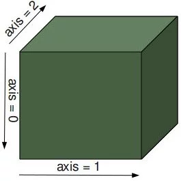
Two- and Multidimensional Arrays
Of course, arrays of NumPy are not limited to one dimension. They are of arbitrary dimension. We create them by passing nested lists (or tuples) to the array method of numpy.
A = np.array([ [3.4, 8.7, 9.9],
               [1.1, -7.8, -0.7],
               [4.1, 12.3, 4.8]])
print(A)
print(A.ndim)
OUTPUT:
[[ 3.4  8.7  9.9]
 [ 1.1 -7.8 -0.7]
 [ 4.1 12.3  4.8]]
2
B = np.array([ [[111, 112], [121, 122]],
               [[211, 212], [221, 222]],
               [[311, 312], [321, 322]] ])
print(B)
print(B.ndim)
OUTPUT:
[[[111 112]
  [121 122]]

 [[211 212]
  [221 222]]

 [[311 312]
  [321 322]]]
3
Shape of an Array
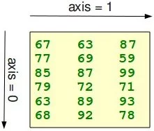
The function "shape" returns the shape of an array. The shape is a tuple of integers. These numbers denote the lengths of the corresponding array dimension. In other words: The "shape" of an array is a tuple with the number of elements per axis (dimension). In our example, the shape is equal to (6, 3), i.e. we have 6 lines and 3 columns.
x = np.array([ [67, 63, 87],
               [77, 69, 59],
               [85, 87, 99],
               [79, 72, 71],
               [63, 89, 93],
               [68, 92, 78]])

print(np.shape(x))
OUTPUT:
(6, 3)
There is also an equivalent array property:
print(x.shape)
OUTPUT:
(6, 3)
The shape of an array tells us also something about the order in which the indices are processed, i.e. first rows, then columns and after that the further dimensions.
"shape" can also be used to change the shape of an array.
x.shape = (3, 6)
print(x)
OUTPUT:
[[67 63 87 77 69 59]
 [85 87 99 79 72 71]
 [63 89 93 68 92 78]]
x.shape = (2, 9)
print(x)
OUTPUT:
[[67 63 87 77 69 59 85 87 99]
 [79 72 71 63 89 93 68 92 78]]
You might have guessed by now that the new shape must correspond to the number of elements of the array, i.e. the total size of the new array must be the same as the old one. We will raise an exception, if this is not the case.
Let's look at some further examples.
The shape of a scalar is an empty tuple:
x = np.array(11)
print(np.shape(x))
OUTPUT:
()
B = np.array([ [[111, 112, 113], [121, 122, 123]],
               [[211, 212, 213], [221, 222, 223]],
               [[311, 312, 313], [321, 322, 323]],
               [[411, 412, 413], [421, 422, 423]] ])

print(B.shape)
OUTPUT:
(4, 2, 3)
Live Python training
Enjoying this page? We offer live Python training courses covering the content of this site.
See our Python training courses
Indexing and Slicing
Assigning to and accessing the elements of an array is similar to other sequential data types of Python, i.e. lists and tuples. We have also many options to indexing, which makes indexing in Numpy very powerful and similar to the indexing of lists and tuples.
Single indexing behaves the way, you will most probably expect it:
F = np.array([1, 1, 2, 3, 5, 8, 13, 21])
# print the first element of F
print(F[0])
# print the last element of F
print(F[-1])
OUTPUT:
1
21
Indexing multidimensional arrays:
A = np.array([ [3.4, 8.7, 9.9],
               [1.1, -7.8, -0.7],
               [4.1, 12.3, 4.8]])

print(A[1][0])
OUTPUT:
1.1
We accessed an element in the second row, i.e. the row with the index 1, and the first column (index 0). We accessed it the same way, we would have done with an element of a nested Python list.
You have to be aware of the fact, that way of accessing multi-dimensional arrays can be highly inefficient. The reason is that we create an intermediate array A[1] from which we access the element with the index 0. So it behaves similar to this:
tmp = A[1]
print(tmp)
print(tmp[0])
OUTPUT:
[ 1.1 -7.8 -0.7]
1.1
There is another way to access elements of multi-dimensional arrays in Numpy: We use only one pair of square brackets and all the indices are separated by commas:
print(A[1, 0])
OUTPUT:
1.1
We assume that you are familar with the slicing of lists and tuples. The syntax is the same in numpy for one-dimensional arrays, but it can be applied to multiple dimensions as well.
The general syntax for a one-dimensional array A looks like this:
A[start:stop:step]
We illustrate the operating principle of "slicing" with some examples. We start with the easiest case, i.e. the slicing of a one-dimensional array:
S = np.array([0, 1, 2, 3, 4, 5, 6, 7, 8, 9])
print(S[2:5])
print(S[:4])
print(S[6:])
print(S[:])
OUTPUT:
[2 3 4]
[0 1 2 3]
[6 7 8 9]
[0 1 2 3 4 5 6 7 8 9]
We will illustrate the multidimensional slicing in the following examples. The ranges for each dimension are separated by commas:
A = np.array([
[11, 12, 13, 14, 15],
[21, 22, 23, 24, 25],
[31, 32, 33, 34, 35],
[41, 42, 43, 44, 45],
[51, 52, 53, 54, 55]])
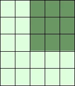
print(A[:3, 2:])
OUTPUT:
[[13 14 15]
 [23 24 25]
 [33 34 35]]
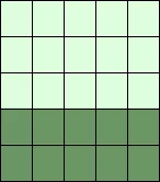
print(A[3:, :])
OUTPUT:
[[41 42 43 44 45]
 [51 52 53 54 55]]
print(A[:, 4:])
OUTPUT:
[[15]
 [25]
 [35]
 [45]
 [55]]
The following two examples use the third parameter "step". The reshape function is used to construct the two-dimensional array. We will explain reshape in the following subchapter:
X = np.arange(28).reshape(4, 7)
print(X)
OUTPUT:
[[ 0  1  2  3  4  5  6]
 [ 7  8  9 10 11 12 13]
 [14 15 16 17 18 19 20]
 [21 22 23 24 25 26 27]]
print(X[::2, ::3])
OUTPUT:
[[ 0  3  6]
 [14 17 20]]
print(X[::, ::3])
OUTPUT:
[[ 0  3  6]
 [ 7 10 13]
 [14 17 20]
 [21 24 27]]

If the number of objects in the selection tuple is less than the dimension N, then : is assumed for any subsequent dimensions:
A = np.array(
    [ [ [45, 12, 4], [45, 13, 5], [46, 12, 6] ],
      [ [46, 14, 4], [45, 14, 5], [46, 11, 5] ],
      [ [47, 13, 2], [48, 15, 5], [52, 15, 1] ] ])

A[1:3, 0:2]  # equivalent to A[1:3, 0:2, :]
OUTPUT:
array([[[46, 14,  4],
        [45, 14,  5]],

       [[47, 13,  2],
        [48, 15,  5]]])
Attention: Whereas slicings on lists and tuples create new objects, a slicing operation on an array creates a view on the original array. So we get an another possibility to access the array, or better a part of the array. From this follows that if we modify a view, the original array will be modified as well.
A = np.array([0, 1, 2, 3, 4, 5, 6, 7, 8, 9])
S = A[2:6]
S[0] = 22
S[1] = 23
print(A)
OUTPUT:
[ 0 1 22 23 4 5 6 7 8 9]
Doing the similar thing with lists, we can see that we get a copy:
lst = [0, 1, 2, 3, 4, 5, 6, 7, 8, 9]
lst2 = lst[2:6]
lst2[0] = 22
lst2[1] = 23
print(lst)
OUTPUT:
[0, 1, 2, 3, 4, 5, 6, 7, 8, 9]
If you want to check, if two array names share the same memory block, you can use the function np.may_share_memory.
np.may_share_memory(A, B)
To determine if two arrays A and B can share memory the memory-bounds of A and B are computed. The function returns True, if they overlap and False otherwise. The function may give false positives, i.e. if it returns True it just means that the arrays may be the same.
np.may_share_memory(A, S)
OUTPUT:
True
The following code shows a case, in which the use of may_share_memory is quite useful:
A = np.arange(12)
B = A.reshape(3, 4)
A[0] = 42
print(B)
OUTPUT:
[[42  1  2  3]
 [ 4  5  6  7]
 [ 8  9 10 11]]
We can see that A and B share the memory in some way. The array attribute "data" is an object pointer to the start of an array's data.
But we saw that if we change an element of one array the other one is changed as well. This fact is reflected by may_share_memory:
np.may_share_memory(A, B)
OUTPUT:
True
The result above is "false positive" example for may_share_memory in the sense that somebody may think that the arrays are the same, which is not the case.
Creating Arrays with Ones, Zeros and Empty
There are two ways of initializing Arrays with Zeros or Ones. The method ones(t) takes a tuple t with the shape of the array and fills the array accordingly with ones. By default it will be filled with Ones of type float. If you need integer Ones, you have to set the optional parameter dtype to int:
import numpy as np

E = np.ones((2,3))
print(E)

F = np.ones((3,4),dtype=int)
print(F)
OUTPUT:
[[1. 1. 1.]
 [1. 1. 1.]]
[[1 1 1 1]
 [1 1 1 1]
 [1 1 1 1]]
What we have said about the method ones() is valid for the method zeros() analogously, as we can see in the following example:
Z = np.zeros((2,4))
print(Z)
OUTPUT:
[[0. 0. 0. 0.]
 [0. 0. 0. 0.]]
There is another interesting way to create an array with Ones or with Zeros, if it has to have the same shape as another existing array 'a'. Numpy supplies for this purpose the methods ones_like(a) and zeros_like(a).
x = np.array([2,5,18,14,4])
E = np.ones_like(x)
print(E)

Z = np.zeros_like(x)
print(Z)
OUTPUT:
[1 1 1 1 1]
[0 0 0 0 0]
There is also a way of creating an array with the empty function. It creates and returns a reference to a new array of given shape and type, without initializing the entries. Sometimes the entries are zeros, but you shouldn't be mislead. Usually, they are arbitrary values.
np.empty((2, 4))
OUTPUT:
array([[0., 0., 0., 0.],
       [0., 0., 0., 0.]])
Live Python training
Enjoying this page? We offer live Python training courses covering the content of this site.
See our Python training courses
Copying Arrays
numpy.copy()
copy(obj, order='K')
Return an array copy of the given object 'obj'.
| Parameter | Meaning |
|---|---|
| obj | array_like input data. |
| order | The possible values are {'C', 'F', 'A', 'K'}. This parameter controls the memory layout of the copy. 'C' means C-order, 'F' means Fortran-order, 'A' means 'F' if the object 'obj' is Fortran contiguous, 'C' otherwise. 'K' means match the layout of 'obj' as closely as possible. |
import numpy as np

x = np.array([[42,22,12],[44,53,66]], order='F')
y = x.copy()

x[0,0] = 1001
print(x)

print(y)
OUTPUT:
[[1001   22   12]
 [  44   53   66]]
[[42 22 12]
 [44 53 66]]
print(x.flags['C_CONTIGUOUS'])
print(y.flags['C_CONTIGUOUS'])
OUTPUT:
False
True
ndarray.copy()
There is also a ndarray method 'copy', which can be directly applied to an array. It is similiar to the above function, but the default values for the order arguments are different.
a.copy(order='C')
Returns a copy of the array 'a'.
| Parameter | Meaning |
|---|---|
| order | The same as with numpy.copy, but 'C' is the default value for order. |
import numpy as np

x = np.array([[42,22,12],[44,53,66]], order='F')
y = x.copy()
x[0,0] = 1001
print(x)

print(y)

print(x.flags['C_CONTIGUOUS'])
print(y.flags['C_CONTIGUOUS'])
OUTPUT:
[[1001   22   12]
 [  44   53   66]]
[[42 22 12]
 [44 53 66]]
False
True
Identity Array
In linear algebra, the identity matrix, or unit matrix, of size n is the n × n square matrix with ones on the main diagonal and zeros elsewhere.
There are two ways in Numpy to create identity arrays:
- identy
- eye
The identity Function
We can create identity arrays with the function identity:
identity(n, dtype=None)
The parameters:
| Parameter | Meaning |
|---|---|
| n | An integer number defining the number of rows and columns of the output, i.e. 'n' x 'n' |
| dtype | An optional argument, defining the data-type of the output. The default is 'float' |
The output of identity is an 'n' x 'n' array with its main diagonal set to one, and all other elements are 0.
import numpy as np

np.identity(4)
OUTPUT:
array([[1., 0., 0., 0.],
       [0., 1., 0., 0.],
       [0., 0., 1., 0.],
       [0., 0., 0., 1.]])
np.identity(4, dtype=int) # equivalent to np.identity(3, int)
OUTPUT:
array([[1, 0, 0, 0],
       [0, 1, 0, 0],
       [0, 0, 1, 0],
       [0, 0, 0, 1]])
The eye Function
Another way to create identity arrays provides the function eye. This function creates also diagonal arrays consisting solely of ones.
It returns a 2-D array with ones on the diagonal and zeros elsewhere.
eye(N, M=None, k=0, dtype=float)
| Parameter | Meaning |
|---|---|
| N | An integer number defining the rows of the output array. |
| M | An optional integer for setting the number of columns in the output. If it is None, it defaults to 'N'. |
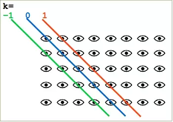
| k | Defining the position of the diagonal. The default is 0. 0 refers to the main diagonal. A positive value refers to an upper diagonal, and a negative value to a lower diagonal. |
| dtype | Optional data-type of the returned array. |
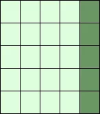
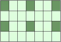
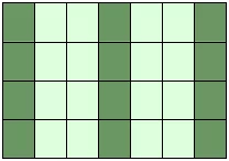
eye returns an ndarray of shape (N,M). All elements of this array are equal to zero, except for the 'k'-th diagonal, whose values are equal to one.
import numpy as np

np.eye(5, 8, k=1, dtype=int)
OUTPUT:
array([[0, 1, 0, 0, 0, 0, 0, 0],
       [0, 0, 1, 0, 0, 0, 0, 0],
       [0, 0, 0, 1, 0, 0, 0, 0],
       [0, 0, 0, 0, 1, 0, 0, 0],
       [0, 0, 0, 0, 0, 1, 0, 0]])
The principle of operation of the parameter 'd' of the eye function is illustrated in the following diagram:
Live Python training
Enjoying this page? We offer live Python training courses covering the content of this site.
See our Python training courses
Exercises:
1) Create an arbitrary one dimensional array called "v".
2) Create a new array which consists of the odd indices of previously created array "v".
3) Create a new array in backwards ordering from v.
4) What will be the output of the following code:
   a = np.array([1, 2, 3, 4, 5])
   b = a[1:4]
   b[0] = 200
   print(a[1])
5) Create a two dimensional array called "m".
6) Create a new array from m, in which the elements of each row are in reverse order.
7) Another one, where the rows are in reverse order.
8) Create an array from m, where columns and rows are in reverse order.
9) Cut of the first and last row and the first and last column.
Solutions to the Exercises:
1)
   import numpy as np
   a = np.array([3,8,12,18,7,11,30])
2)
odd_elements = a[1::2]
3) reverse_order = a[::-1]
4) The output will be 200, because slices are views in numpy and not copies.
5) m = np.array([ [11, 12, 13, 14], [21, 22, 23, 24], [31, 32, 33, 34]])
6) m[::,::-1]
7) m[::-1]
8) m[::-1,::-1]
9) m[1:-1,1:-1]
Live Python training
Enjoying this page? We offer live Python training courses covering the content of this site.
Upcoming online Courses
See our Python training courses