22. Neural Networks with Scikit
By Bernd Klein. Last modified: 19 Apr 2024.
Introduction

In the previous chapters of our tutorial, we manually created Neural Networks. This was necessary to get a deep understanding of how Neural networks can be implemented. This understanding is very useful to use the classifiers provided by the sklearn module of Python. In this chapter we will use the multilayer perceptron classifier MLPClassifier contained in sklearn.neural_network
We will use again the Iris dataset, which we had used already multiple times in our Machine Learning tutorial with Python, to introduce this classifier.
Live Python training

Enjoying this page? We offer live Python training courses covering the content of this site.
See our Python training courses
MLPClassifier classifier
We will continue with examples using the multilayer perceptron (MLP). The multilayer perceptron (MLP) is a feedforward artificial neural network model that maps sets of input data onto a set of appropriate outputs. An MLP consists of multiple layers and each layer is fully connected to the following one. The nodes of the layers are neurons using nonlinear activation functions, except for the nodes of the input layer. There can be one or more non-linear hidden layers between the input and the output layer.
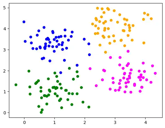
Multilabel Example
import matplotlib.pyplot as plt
from sklearn.datasets import make_blobs

n_samples = 200
blob_centers = ([1, 1], [3, 4], [1, 3.3], [3.5, 1.8])
data, labels = make_blobs(n_samples=n_samples,
                          centers=blob_centers,
                          cluster_std=0.5,
                          random_state=0)


colours = ('green', 'orange', "blue", "magenta")
fig, ax = plt.subplots()

for n_class in range(len(blob_centers)):
    ax.scatter(data[labels==n_class][:, 0],
               data[labels==n_class][:, 1],
               c=colours[n_class],
               s=30,
               label=str(n_class))
from sklearn.model_selection import train_test_split
datasets = train_test_split(data,
                            labels,
                            test_size=0.2)

train_data, test_data, train_labels, test_labels = datasets
We will create now a MLPClassifier.
A few notes on the used parameters:
- hidden_layer_sizes: tuple, length = n_layers - 2, default=(100,)
The ith element represents the number of neurons in the ith hidden layer.
(6,)means one hidden layer with 6 neurons -
solver:
The weight optimization can be influenced with the
solverparameter. Three solver modes are available- 'lbfgs'
is an optimizer in the family of quasi-Newton methods. - 'sgd'
refers to stochastic gradient descent. - 'adam' refers to a stochastic gradient-based optimizer proposed by Kingma, Diederik, and Jimmy Ba
Without understanding in the details of the solvers, you should know the following: 'adam' works pretty well - both training time and validation score - on relatively large datasets, i.e. thousands of training samples or more. For small datasets, however, 'lbfgs' can converge faster and perform better.
- 'lbfgs'
-
'alpha'
This parameter can be used to control possible 'overfitting' and 'underfitting'. We will cover it in detail further down in this chapter.
from sklearn.neural_network import MLPClassifier

clf = MLPClassifier(solver='lbfgs',
                    alpha=1e-5,
                    hidden_layer_sizes=(6,),
                    random_state=1)

clf.fit(train_data, train_labels)
OUTPUT:
MLPClassifier(alpha=1e-05, hidden_layer_sizes=(6,), random_state=1,
              solver='lbfgs')MLPClassifier(alpha=1e-05, hidden_layer_sizes=(6,), random_state=1,
              solver='lbfgs')
clf.score(train_data, train_labels)
OUTPUT:
1.0
from sklearn.metrics import accuracy_score

predictions_train = clf.predict(train_data)
predictions_test = clf.predict(test_data)
train_score = accuracy_score(predictions_train, train_labels)
print("score on train data: ", train_score)
test_score = accuracy_score(predictions_test, test_labels)
print("score on test data: ", test_score)
OUTPUT:
score on train data:  1.0
score on test data:  0.975
predictions_train[:20]
OUTPUT:
array([2, 3, 3, 0, 2, 0, 2, 0, 3, 0, 2, 1, 3, 3, 3, 3, 0, 2, 3, 1])
Multi-layer Perceptron
from sklearn.neural_network import MLPClassifier
X = [[0., 0.], [0., 1.], [1., 0.], [1., 1.]]
y = [0, 0, 0, 1]
clf = MLPClassifier(solver='lbfgs', alpha=1e-5,
                    hidden_layer_sizes=(5, 2), random_state=1)

print(clf.fit(X, y))
OUTPUT:
MLPClassifier(alpha=1e-05, hidden_layer_sizes=(5, 2), random_state=1,
              solver='lbfgs')
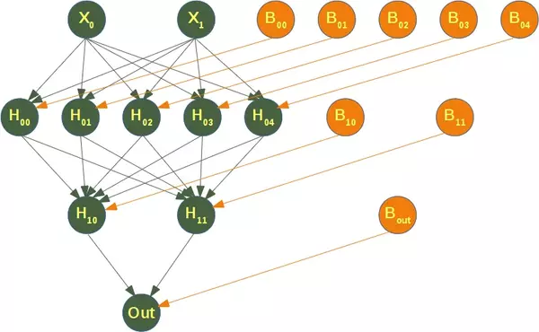
The following diagram depicts the neural network, that we have trained for our classifier clf. We have two input nodes $X_0$ and $X_1$, called the input layer, and one output neuron 'Out'. We have two hidden layers the first one with the neurons $H_{00}$ ... $H_{04}$ and the second hidden layer consisting of $H_{10}$ and $H_{11}$. Each neuron of the hidden layers and the output neuron possesses a corresponding Bias, i.e. $B_{00}$ is the corresponding Bias to the neuron $H_{00}$, $B_{01}$ is the corresponding Bias to the neuron $H_{01}$ and so on.
Each neuron of the hidden layers receives the output from every neuron of the previous layers and transforms these values with a weighted linear summation
into an output value, where n is the number of neurons of the layer and $w_i$ corresponds to the ith component of the weight vector. The output layer receives the values from the last hidden layer. It also performs a linear summation, but a non-linear activation function
like the hyperbolic tan function will be applied to the summation result.
The attribute coefs_ contains a list of weight matrices for every layer. The weight matrix at index i holds the weights between the layer i and layer i + 1.
print("weights between input and first hidden layer:")
print(clf.coefs_[0])
print("\nweights between first hidden and second hidden layer:")
print(clf.coefs_[1])
OUTPUT:
weights between input and first hidden layer:
[[-0.14203691 -1.18304359 -0.85567518 -4.53250719 -0.60466275]
 [-0.69781111 -3.5850093  -0.26436018 -4.39161248  0.06644423]]

weights between first hidden and second hidden layer:
[[ 0.29179638 -0.14155284]
 [ 4.02666592 -0.61556475]
 [-0.51677234  0.51479708]
 [ 7.37215202 -0.31936965]
 [ 0.32920668  0.64428109]]
The summation formula of the neuron H00 is defined by:
which can be written as
because $B_{11} = 1$.
We can get the values for $w_0$ and $w_1$ from clf.coefs_ like this:
$w_0 =$ clf.coefs_[0][0][0] and $w_1 =$ clf.coefs_[0][1][0]
print("w0 = ", clf.coefs_[0][0][0])
print("w1 = ", clf.coefs_[0][1][0])
OUTPUT:
w0 =  -0.14203691267827162
w1 =  -0.6978111149778686
The weight vector of $H_{00}$ can be accessed with
clf.coefs_[0][:,0]
OUTPUT:
array([-0.14203691, -0.69781111])
We can generalize the above to access a neuron $H_{ij}$ in the following way:
for i in range(len(clf.coefs_)):
    number_neurons_in_layer = clf.coefs_[i].shape[1]
    for j in range(number_neurons_in_layer):
        weights = clf.coefs_[i][:,j]
        print(i, j, weights, end=", ")
        print()
    print()
OUTPUT:
0 0 [-0.14203691 -0.69781111],
0 1 [-1.18304359 -3.5850093 ],
0 2 [-0.85567518 -0.26436018],
0 3 [-4.53250719 -4.39161248],
0 4 [-0.60466275  0.06644423],

1 0 [ 0.29179638  4.02666592 -0.51677234  7.37215202  0.32920668],
1 1 [-0.14155284 -0.61556475  0.51479708 -0.31936965  0.64428109],

2 0 [-4.96774269 -0.86330397],
intercepts_ is a list of bias vectors, where the vector at index i represents the bias values added to layer i+1.
print("Bias values for first hidden layer:")
print(clf.intercepts_[0])
print("\nBias values for second hidden layer:")
print(clf.intercepts_[1])
OUTPUT:
Bias values for first hidden layer:
[-0.14962269 -0.59232707 -0.5472481   7.02667699 -0.87510813]

Bias values for second hidden layer:
[-3.61417672 -0.76834882]
The main reason, why we train a classifier is to predict results for new samples. We can do this with the predict method. The method returns a predicted class for a sample, in our case a "0" or a "1" :
result = clf.predict([[0, 0], [0, 1],
                      [1, 0], [0, 1],
                      [1, 1], [2., 2.],
                      [1.3, 1.3], [2, 4.8]])
Instead of just looking at the class results, we can also use the predict_proba method to get the probability estimates.
prob_results = clf.predict_proba([[0, 0], [0, 1],
                                  [1, 0], [0, 1],
                                  [1, 1], [2., 2.],
                                  [1.3, 1.3], [2, 4.8]])
print(prob_results)
OUTPUT:
[[1.00000000e+000 5.25723951e-101]
 [1.00000000e+000 3.71534882e-031]
 [1.00000000e+000 6.47069178e-029]
 [1.00000000e+000 3.71534882e-031]
 [2.07145538e-004 9.99792854e-001]
 [2.07145538e-004 9.99792854e-001]
 [2.07145538e-004 9.99792854e-001]
 [2.07145538e-004 9.99792854e-001]]
prob_results[i][0] gives us the probability for the class0, i.e. a "0" and results[i][1] the probabilty for a "1". i corresponds to the ith sample.
Live Python training
Enjoying this page? We offer live Python training courses covering the content of this site.
Upcoming online Courses
See our Python training courses
Complete Iris Dataset Example
from sklearn.datasets import load_iris

iris = load_iris()
# splitting into train and test datasets

from sklearn.model_selection import train_test_split
datasets = train_test_split(iris.data, iris.target,
                            test_size=0.2)

train_data, test_data, train_labels, test_labels = datasets
# scaling the data
from sklearn.preprocessing import StandardScaler
scaler = StandardScaler()

# we fit the train data
scaler.fit(train_data)

# scaling the train data
train_data = scaler.transform(train_data)
test_data = scaler.transform(test_data)

print(train_data[:3])
OUTPUT:
[[-0.53115203  2.01478627 -1.1949835  -1.05266199]
 [ 1.3398336   0.14238083  0.76937294  1.46049962]
 [-0.78061678  1.07858355 -1.31053388 -1.31720532]]
# Training the Model
from sklearn.neural_network import MLPClassifier
# creating an classifier from the model:
mlp = MLPClassifier(hidden_layer_sizes=(10, 5), max_iter=1000)

# let's fit the training data to our model
mlp.fit(train_data, train_labels)
OUTPUT:
MLPClassifier(hidden_layer_sizes=(10, 5), max_iter=1000)MLPClassifier(hidden_layer_sizes=(10, 5), max_iter=1000)
from sklearn.metrics import accuracy_score

predictions_train = mlp.predict(train_data)
print(accuracy_score(predictions_train, train_labels))
predictions_test = mlp.predict(test_data)
print(accuracy_score(predictions_test, test_labels))
OUTPUT:
0.975
1.0
from sklearn.metrics import confusion_matrix

confusion_matrix(predictions_train, train_labels)
OUTPUT:
array([[39,  0,  0],
       [ 0, 40,  1],
       [ 0,  2, 38]])
confusion_matrix(predictions_test, test_labels)
OUTPUT:
array([[11,  0,  0],
       [ 0,  8,  0],
       [ 0,  0, 11]])
from sklearn.metrics import classification_report

print(classification_report(predictions_test, test_labels))
OUTPUT:
              precision    recall  f1-score   support

           0       1.00      1.00      1.00        11
           1       1.00      1.00      1.00         8
           2       1.00      1.00      1.00        11

    accuracy                           1.00        30
   macro avg       1.00      1.00      1.00        30
weighted avg       1.00      1.00      1.00        30
MNIST Dataset
We have already used the MNIST dataset in the chapter Testing with MNIST of our tutorial. You will also find some explanations about this dataset.
We want to apply the MLPClassifier on the MNIST data. We can load in the data with pickle:
import pickle

with open("../data/mnist/pickled_mnist.pkl", "br") as fh:
    data = pickle.load(fh)

data
OUTPUT:
(array([[0.01, 0.01, 0.01, ..., 0.01, 0.01, 0.01],
        [0.01, 0.01, 0.01, ..., 0.01, 0.01, 0.01],
        [0.01, 0.01, 0.01, ..., 0.01, 0.01, 0.01],
        ...,
        [0.01, 0.01, 0.01, ..., 0.01, 0.01, 0.01],
        [0.01, 0.01, 0.01, ..., 0.01, 0.01, 0.01],
        [0.01, 0.01, 0.01, ..., 0.01, 0.01, 0.01]]),
 array([[0.01, 0.01, 0.01, ..., 0.01, 0.01, 0.01],
        [0.01, 0.01, 0.01, ..., 0.01, 0.01, 0.01],
        [0.01, 0.01, 0.01, ..., 0.01, 0.01, 0.01],
        ...,
        [0.01, 0.01, 0.01, ..., 0.01, 0.01, 0.01],
        [0.01, 0.01, 0.01, ..., 0.01, 0.01, 0.01],
        [0.01, 0.01, 0.01, ..., 0.01, 0.01, 0.01]]),
 array([[5.],
        [0.],
        [4.],
        ...,
        [5.],
        [6.],
        [8.]]),
 array([[7.],
        [2.],
        [1.],
        ...,
        [4.],
        [5.],
        [6.]]))
train_imgs = data[0]
test_imgs = data[1]
train_labels = data[2]
test_labels = data[3]

image_size = 28 # width and length
no_of_different_labels = 10 #  i.e. 0, 1, 2, 3, ..., 9
image_pixels = image_size * image_size
mlp = MLPClassifier(hidden_layer_sizes=(100, ),
                    max_iter=480, alpha=1e-4,
                    solver='sgd', verbose=10,
                    tol=1e-4, random_state=1,
                    learning_rate_init=.1)

train_labels = train_labels.reshape(train_labels.shape[0],)
print(train_imgs.shape, train_labels.shape)

mlp.fit(train_imgs, train_labels)
print("Training set score: %f" % mlp.score(train_imgs, train_labels))
print("Test set score: %f" % mlp.score(test_imgs, test_labels))
OUTPUT:
(60000, 784) (60000,)
Iteration 1, loss = 0.29753549
Iteration 2, loss = 0.12369769
Iteration 3, loss = 0.08872688
Iteration 4, loss = 0.07084598
Iteration 5, loss = 0.05874947
Iteration 6, loss = 0.04876359
Iteration 7, loss = 0.04203350
Iteration 8, loss = 0.03525624
Iteration 9, loss = 0.02995642
Iteration 10, loss = 0.02526208
Iteration 11, loss = 0.02195436
Iteration 12, loss = 0.01825246
Iteration 13, loss = 0.01543440
Iteration 14, loss = 0.01320164
Iteration 15, loss = 0.01057486
Iteration 16, loss = 0.00984482
Iteration 17, loss = 0.00776886
Iteration 18, loss = 0.00655891
Iteration 19, loss = 0.00539189
Iteration 20, loss = 0.00460981
Iteration 21, loss = 0.00396910
Iteration 22, loss = 0.00350800
Iteration 23, loss = 0.00328115
Iteration 24, loss = 0.00294118
Iteration 25, loss = 0.00265852
Iteration 26, loss = 0.00241809
Iteration 27, loss = 0.00234944
Iteration 28, loss = 0.00215147
Iteration 29, loss = 0.00201855
Iteration 30, loss = 0.00187808
Iteration 31, loss = 0.00183098
Iteration 32, loss = 0.00172363
Iteration 33, loss = 0.00169482
Iteration 34, loss = 0.00159811
Iteration 35, loss = 0.00152427
Iteration 36, loss = 0.00148731
Iteration 37, loss = 0.00144202
Iteration 38, loss = 0.00138101
Iteration 39, loss = 0.00133767
Iteration 40, loss = 0.00130437
Iteration 41, loss = 0.00126314
Iteration 42, loss = 0.00122969
Iteration 43, loss = 0.00119848
Training loss did not improve more than tol=0.000100 for 10 consecutive epochs. Stopping.
Training set score: 1.000000
Test set score: 0.977900
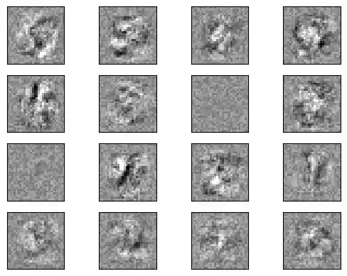
fig, axes = plt.subplots(4, 4)
# use global min / max to ensure all weights are shown on the same scale
vmin, vmax = mlp.coefs_[0].min(), mlp.coefs_[0].max()
for coef, ax in zip(mlp.coefs_[0].T, axes.ravel()):
    ax.matshow(coef.reshape(28, 28), cmap=plt.cm.gray, vmin=.5 * vmin,
               vmax=.5 * vmax)
    ax.set_xticks(())
    ax.set_yticks(())

plt.show()
Live Python training
Enjoying this page? We offer live Python training courses covering the content of this site.
See our Python training courses
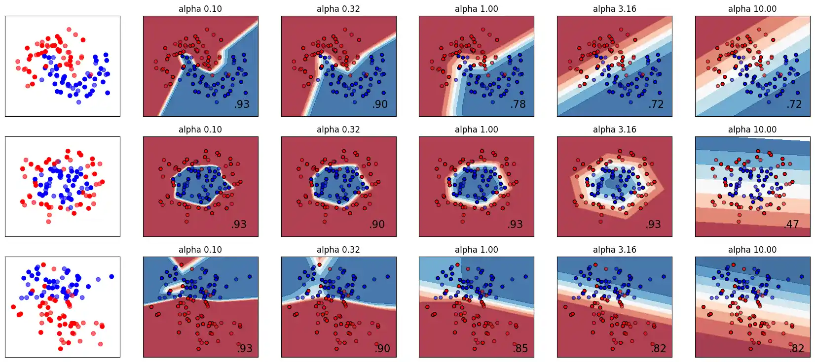
The Parameter alpha
A comparison of different values for regularization parameter ‘alpha’ on synthetic datasets. The plot shows that different alphas yield different decision functions.
Alpha is a parameter for regularization term, aka penalty term, that combats overfitting by constraining the size of the weights. Increasing alpha may fix high variance (a sign of overfitting) by encouraging smaller weights, resulting in a decision boundary plot that appears with lesser curvatures. Similarly, decreasing alpha may fix high bias (a sign of underfitting) by encouraging larger weights, potentially resulting in a more complicated decision boundary.
# Author: Issam H. Laradji
# License: BSD 3 clause
# code from: https://scikit-learn.org/stable/auto_examples/neural_networks/plot_mlp_alpha.html

import numpy as np
from matplotlib import pyplot as plt
from matplotlib.colors import ListedColormap
from sklearn.model_selection import train_test_split
from sklearn.preprocessing import StandardScaler
from sklearn.datasets import make_moons, make_circles, make_classification
from sklearn.neural_network import MLPClassifier
from sklearn.pipeline import make_pipeline

h = .02  # step size in the mesh

alphas = np.logspace(-1, 1, 5)

classifiers = []
names = []
for alpha in alphas:
    classifiers.append(make_pipeline(
        StandardScaler(),
        MLPClassifier(
            solver='lbfgs', alpha=alpha, random_state=1, max_iter=2000,
            early_stopping=True, hidden_layer_sizes=[100, 100],
        )
    ))
    names.append(f"alpha {alpha:.2f}")

X, y = make_classification(n_features=2, n_redundant=0, n_informative=2,
                           random_state=0, n_clusters_per_class=1)
rng = np.random.RandomState(2)
X += 2 * rng.uniform(size=X.shape)
linearly_separable = (X, y)

datasets = [make_moons(noise=0.3, random_state=0),
            make_circles(noise=0.2, factor=0.5, random_state=1),
            linearly_separable]

figure = plt.figure(figsize=(17, 9))
i = 1
# iterate over datasets
for X, y in datasets:
    # split into training and test part
    X_train, X_test, y_train, y_test = train_test_split(X, y, test_size=.4)

    x_min, x_max = X[:, 0].min() - .5, X[:, 0].max() + .5
    y_min, y_max = X[:, 1].min() - .5, X[:, 1].max() + .5
    xx, yy = np.meshgrid(np.arange(x_min, x_max, h),
                         np.arange(y_min, y_max, h))

    # just plot the dataset first
    cm = plt.cm.RdBu
    cm_bright = ListedColormap(['#FF0000', '#0000FF'])
    ax = plt.subplot(len(datasets), len(classifiers) + 1, i)
    # Plot the training points
    ax.scatter(X_train[:, 0], X_train[:, 1], c=y_train, cmap=cm_bright)
    # and testing points
    ax.scatter(X_test[:, 0], X_test[:, 1], c=y_test, cmap=cm_bright, alpha=0.6)
    ax.set_xlim(xx.min(), xx.max())
    ax.set_ylim(yy.min(), yy.max())
    ax.set_xticks(())
    ax.set_yticks(())
    i += 1

    # iterate over classifiers
    for name, clf in zip(names, classifiers):
        ax = plt.subplot(len(datasets), len(classifiers) + 1, i)
        clf.fit(X_train, y_train)
        score = clf.score(X_test, y_test)

        # Plot the decision boundary. For that, we will assign a color to each
        # point in the mesh [x_min, x_max] x [y_min, y_max].
        if hasattr(clf, "decision_function"):
            Z = clf.decision_function(np.c_[xx.ravel(), yy.ravel()])
        else:
            Z = clf.predict_proba(np.c_[xx.ravel(), yy.ravel()])[:, 1]

        # Put the result into a color plot
        Z = Z.reshape(xx.shape)
        ax.contourf(xx, yy, Z, cmap=cm, alpha=.8)

        # Plot also the training points
        ax.scatter(X_train[:, 0], X_train[:, 1], c=y_train, cmap=cm_bright,
                   edgecolors='black', s=25)
        # and testing points
        ax.scatter(X_test[:, 0], X_test[:, 1], c=y_test, cmap=cm_bright,
                   alpha=0.6, edgecolors='black', s=25)

        ax.set_xlim(xx.min(), xx.max())
        ax.set_ylim(yy.min(), yy.max())
        ax.set_xticks(())
        ax.set_yticks(())
        ax.set_title(name)
        ax.text(xx.max() - .3, yy.min() + .3, ('%.2f' % score).lstrip('0'),
                size=15, horizontalalignment='right')
        i += 1

figure.subplots_adjust(left=.02, right=.98)
plt.show()
Exercises
Exercise 1
Classify the data in "strange_flowers.txt" with a Neural Network.
Exercise 2
Binary Classification with MLPClassifier: Train an MLPClassifier model to classify whether a given tumor is malignant or benign based on tumor features. Use the data from sklearn.
Exercise 3
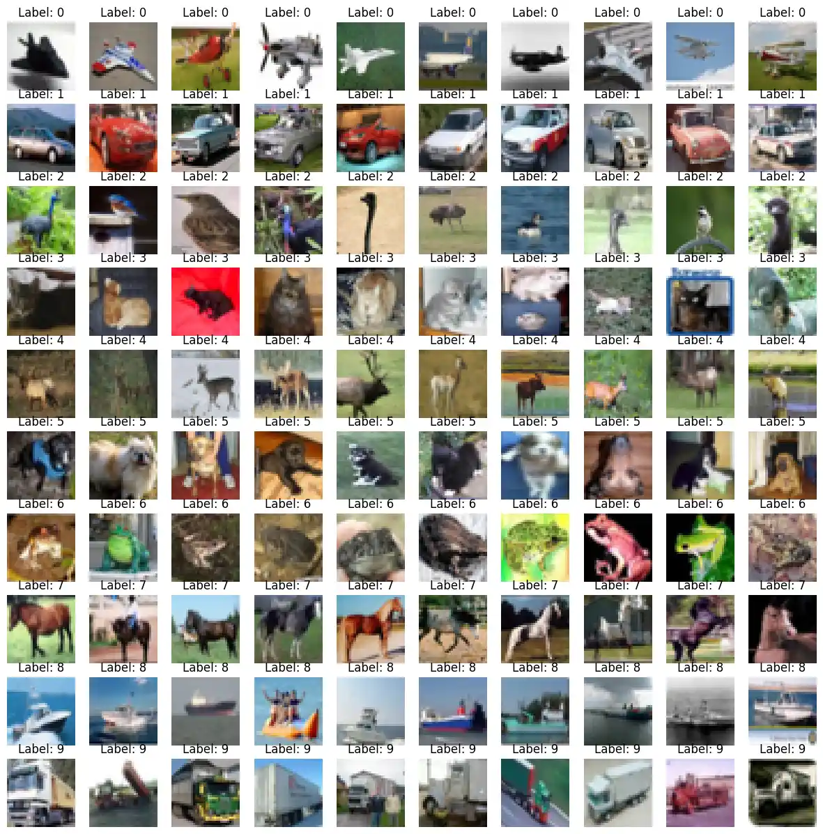
We will use the CIFAR-10 dataset. It is a widely used dataset in the field of machine learning and computer vision.
The CIFAR-10 dataset consists of 60000 32x32 colour images in 10 classes, with 6000 images per class. There are 50000 training images and 10000 test images.
Live Python training
Enjoying this page? We offer live Python training courses covering the content of this site.
See our Python training courses
Solutions
Solution to Exercise 1
We use read_csv of the pandas module to read in the strange_flowers.txt file:
import pandas as pd

dataset = pd.read_csv("data/strange_flowers.txt",
                      header=None,
                      names=["red", "green", "blue", "size", "label"],
                      sep=" ")
dataset
| red | green | blue | size | label | |
|---|---|---|---|---|---|
| 0 | 252.0 | 96.0 | 10.0 | 3.63 | 1.0 |
| 1 | 249.0 | 115.0 | 10.0 | 3.59 | 1.0 |
| 2 | 235.0 | 107.0 | 0.0 | 3.81 | 1.0 |
| 3 | 255.0 | 110.0 | 6.0 | 3.91 | 1.0 |
| 4 | 247.0 | 104.0 | 8.0 | 3.41 | 1.0 |
| ... | ... | ... | ... | ... | ... |
| 790 | 197.0 | 250.0 | 108.0 | 2.69 | 4.0 |
| 791 | 197.0 | 250.0 | 107.0 | 3.05 | 4.0 |
| 792 | 197.0 | 241.0 | 109.0 | 3.23 | 4.0 |
| 793 | 197.0 | 243.0 | 92.0 | 3.00 | 4.0 |
| 794 | 197.0 | 252.0 | 96.0 | 3.06 | 4.0 |
795 rows × 5 columns
The first four columns contain the data and the last column contains the labels:
data = dataset.drop('label', axis=1)
labels = dataset.label
X_train, X_test, y_train, y_test = train_test_split(data,
                                                    labels,
                                                    random_state=0,
                                                    test_size=0.2)
We have to scale the data now to reduce the biases between the data:
from sklearn.preprocessing import StandardScaler
scaler = StandardScaler()
X_train = scaler.fit_transform(X_train) #  transform
X_test = scaler.transform(X_test) #  transform
from sklearn.neural_network import MLPClassifier

mlp = MLPClassifier(hidden_layer_sizes=(100, ),
                    max_iter=480,
                    alpha=1e-4,
                    solver='sgd',
                    tol=1e-4,
                    random_state=1,
                    learning_rate_init=.1)


mlp.fit(X_train, y_train)
print("Training set score: %f" % mlp.score(X_train, y_train))
print("Test set score: %f" % mlp.score(X_test, y_test))
OUTPUT:
Training set score: 0.966981
Test set score: 0.974843
Solution to Exercise 2
from sklearn.datasets import load_breast_cancer
from sklearn.model_selection import train_test_split
from sklearn.neural_network import MLPClassifier
from sklearn.preprocessing import StandardScaler
from sklearn.metrics import accuracy_score
data = load_breast_cancer()
X = data.data
y = data.target

# Split the dataset into training and testing sets:
X_train, X_test, y_train, y_test = train_test_split(X, y, test_size=0.2, random_state=42)
scaler = StandardScaler()
X_train_scaled = scaler.fit_transform(X_train)
X_test_scaled = scaler.transform(X_test)
mlp = MLPClassifier(hidden_layer_sizes=(100,), max_iter=1000, random_state=42)
mlp.fit(X_train_scaled, y_train)

y_pred = mlp.predict(X_test_scaled)
accuracy = accuracy_score(y_test, y_pred)
print("Accuracy:", accuracy)
OUTPUT:
Accuracy: 0.9736842105263158
Solution to Exercise 3
import numpy as np
import matplotlib.pyplot as plt
import pickle

def load_cifar10_batch(file):
    with open(file, 'rb') as fo:
        data = pickle.load(fo, encoding='bytes')
    return data

def plot_cifar_images(data, labels, num_images_per_class=10):
    classes = np.unique(labels)
    fig, axes = plt.subplots(len(classes), num_images_per_class, figsize=(15, 15))

    for i, cls in enumerate(classes):
        class_indices = np.where(labels == cls)[0][:num_images_per_class]
        for j, idx in enumerate(class_indices):
            image = data[idx]
            image = np.transpose(np.reshape(image, (3, 32, 32)), (1, 2, 0))  # Reshape image from flat to (32,32,3)
            axes[i, j].imshow(image)
            axes[i, j].set_title(f"Label: {cls}")
            axes[i, j].axis('off')
    plt.show()

# Load CIFAR-10 data
batch_data = load_cifar10_batch('../data/cifar-10-batches-py/data_batch_1')
data = batch_data[b'data']
labels = batch_data[b'labels']

# Plot CIFAR images
plot_cifar_images(data, labels, num_images_per_class=10)
import numpy as np
import matplotlib.pyplot as plt
import pickle
def load_cifar10_batch(file):
with open(file, 'rb') as fo:
data = pickle.load(fo, encoding='bytes')
return data
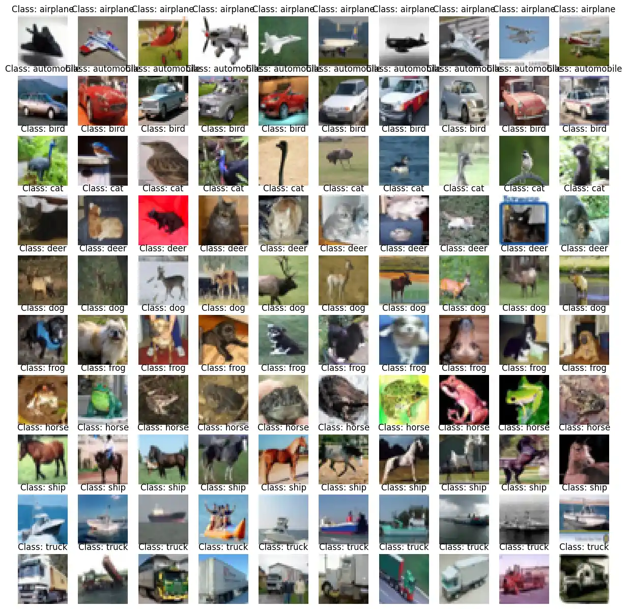
def plot_cifar_images(data, labels, class_names, num_images_per_class=10):
classes = np.unique(labels)
fig, axes = plt.subplots(len(classes), num_images_per_class, figsize=(15, 15))
for i, cls in enumerate(classes):
class_indices = np.where(labels == cls)[0][:num_images_per_class]
for j, idx in enumerate(class_indices):
image = data[idx]
image = np.transpose(np.reshape(image, (3, 32, 32)), (1, 2, 0)) # Reshape image from flat to (32,32,3)
axes[i, j].imshow(image)
axes[i, j].set_title(f"Class: {class_names[cls]}")
axes[i, j].axis('off')
plt.show()
# Load CIFAR-10 data
batch_data = load_cifar10_batch('../data/cifar-10-batches-py/data_batch_1')
data = batch_data[b'data']
labels = batch_data[b'labels']
# Class names for CIFAR-10 dataset
class_names = ['airplane', 'automobile', 'bird', 'cat', 'deer', 'dog', 'frog', 'horse', 'ship', 'truck']
# Plot CIFAR images
plot_cifar_images(data, labels, class_names, num_images_per_class=10)
import numpy as np
import pickle
from sklearn.neural_network import MLPClassifier
from sklearn.preprocessing import StandardScaler
from sklearn.metrics import accuracy_score
from sklearn.metrics import classification_report


def load_cifar10_batch(file):
    with open(file, 'rb') as fo:
        data = pickle.load(fo, encoding='bytes')
    return data

def load_cifar10_data():
    train_data = []
    train_labels = []
    for i in range(1, 6):
        batch_data = load_cifar10_batch('../data/cifar-10-batches-py/data_batch_' + str(i))
        train_data.append(batch_data[b'data'])
        train_labels += batch_data[b'labels']
    train_data = np.concatenate(train_data, axis=0)
    train_labels = np.array(train_labels)

    test_batch = load_cifar10_batch('../data/cifar-10-batches-py/test_batch')
    test_data = test_batch[b'data']
    test_labels = np.array(test_batch[b'labels'])

    return train_data, train_labels, test_data, test_labels

X_train, y_train, X_test, y_test = load_cifar10_data()
scaler = StandardScaler()
X_train_scaled = scaler.fit_transform(X_train)
X_test_scaled = scaler.transform(X_test)
#X_train, X_val, y_train, y_val = train_test_split(X_train, y_train, test_size=0.2, random_state=42)
y_train
OUTPUT:
array([6, 9, 9, ..., 9, 1, 1])
mlp = MLPClassifier(hidden_layer_sizes=(1024, 512, 128), max_iter=500, random_state=42)
mlp.fit(X_train_scaled, y_train)
OUTPUT:
MLPClassifier(hidden_layer_sizes=(1024, 512, 128), max_iter=500,
              random_state=42)MLPClassifier(hidden_layer_sizes=(1024, 512, 128), max_iter=500,
              random_state=42)
y_val_pred = mlp.predict(X_test_scaled)
accuracy = accuracy_score(y_test, y_val_pred)
print("Validation Accuracy:", accuracy)
OUTPUT:
Validation Accuracy: 0.5304
print("Classification Report:")
print(classification_report(y_test, y_val_pred))
OUTPUT:
Classification Report:
              precision    recall  f1-score   support

           0       0.59      0.64      0.61      1000
           1       0.59      0.68      0.63      1000
           2       0.44      0.43      0.43      1000
           3       0.34      0.36      0.35      1000
           4       0.46      0.43      0.45      1000
           5       0.44      0.38      0.40      1000
           6       0.61      0.57      0.59      1000
           7       0.60      0.58      0.59      1000
           8       0.64      0.69      0.66      1000
           9       0.58      0.56      0.57      1000

    accuracy                           0.53     10000
   macro avg       0.53      0.53      0.53     10000
weighted avg       0.53      0.53      0.53     10000
We offer a PyTorch solution without detailed explanation at this time. However, we intend to dedicate a comprehensive chapter to PyTorch, likely in the upcoming autumn:
import torch
import torchvision
import torchvision.transforms as transforms
import torch.nn as nn
import torch.optim as optim
import torch.nn.functional as F

device = (
    "cuda"
    if torch.cuda.is_available()
    else "mps"
    if torch.backends.mps.is_available()
    else "cpu"
)

trainset = torchvision.datasets.CIFAR10(root='./data', train=True, download=True, transform=transforms.ToTensor())
trainloader = torch.utils.data.DataLoader(trainset, batch_size=4, shuffle=True, num_workers=2)

testset = torchvision.datasets.CIFAR10(root='./data', train=False, download=True, transform=transforms.ToTensor())
testloader = torch.utils.data.DataLoader(testset, batch_size=4, shuffle=False, num_workers=2)

classes = ('plane', 'car', 'bird', 'cat', 'deer', 'dog', 'frog', 'horse', 'ship', 'truck')

# Step 2: Define the model
class Net(nn.Module):
    def __init__(self):

        super(Net, self).__init__()
        self.stack = nn.Sequential(
            nn.BatchNorm2d(3), # (subtract average pixel value from each pixel) / variance
            # image size 32 x 32 x 3
            nn.Conv2d(3, 64, 3), #3=RGB, output=64 feature maps, kernelsize= 3 (3*3)
            # image size 30 x 30 x 64
            nn.ReLU(),
            nn.MaxPool2d(2, 2),    # image reduced by 2x2 --> max value
            # image size 15 x 15 x 64
            nn.Conv2d(64, 128, 3),
            nn.ReLU(),
            nn.Conv2d(128, 128, 3),
            # immage size 10 x 10 x 128
            nn.ReLU(),
            nn.MaxPool2d(2, 2),
            # image size 5 x 5 x  128
            nn.Conv2d(128, 256, 3, padding=1, padding_mode='zeros'),
            # image size 5 x 5 x 256
            nn.ReLU(),
            nn.Flatten(),
            # image 6400 = 5*5*256  one dimensional
            nn.Linear(5*5*256, 256),
            nn.ReLU(),
            nn.Linear(256, 10)
        )

    def forward(self, x):
        x = self.stack(x)
        return x

net = Net().to(device)

# Step 3: Define Loss Function and Optimizer
criterion = nn.CrossEntropyLoss()
optimizer = optim.SGD(net.parameters(), lr=0.001, momentum=0.9)

# Step 4-6: Training loop
for epoch in range(10):  # loop over the dataset multiple times

    running_loss = 0.0
    for i, data in enumerate(trainloader, 0):
        inputs, labels = data
        inputs, labels = inputs.to(device), labels.to(device)

        optimizer.zero_grad()

        outputs = net(inputs)
        loss = criterion(outputs, labels)
        loss.backward()
        optimizer.step()

        running_loss += loss.item()
        if i % 2000 == 1999:    # print every 2000 mini-batches
            print('[%d, %5d] loss: %.3f' %
                  (epoch + 1, i + 1, running_loss / 2000))
            running_loss = 0.0

print('Finished Training')
OUTPUT:
Files already downloaded and verified
Files already downloaded and verified
[1,  2000] loss: 2.105
[1,  4000] loss: 1.758
[1,  6000] loss: 1.576
[1,  8000] loss: 1.470
[1, 10000] loss: 1.379
[1, 12000] loss: 1.315
[2,  2000] loss: 1.184
[2,  4000] loss: 1.149
[2,  6000] loss: 1.091
[2,  8000] loss: 1.044
[2, 10000] loss: 1.017
[2, 12000] loss: 0.973
[3,  2000] loss: 0.851
[3,  4000] loss: 0.879
[3,  6000] loss: 0.833
[3,  8000] loss: 0.829
[3, 10000] loss: 0.796
[3, 12000] loss: 0.813
[4,  2000] loss: 0.677
[4,  4000] loss: 0.671
[4,  6000] loss: 0.690
[4,  8000] loss: 0.669
[4, 10000] loss: 0.670
[4, 12000] loss: 0.660
[5,  2000] loss: 0.534
[5,  4000] loss: 0.524
[5,  6000] loss: 0.544
[5,  8000] loss: 0.554
[5, 10000] loss: 0.537
[5, 12000] loss: 0.564
[6,  2000] loss: 0.392
[6,  4000] loss: 0.409
[6,  6000] loss: 0.430
[6,  8000] loss: 0.434
[6, 10000] loss: 0.448
[6, 12000] loss: 0.461
[7,  2000] loss: 0.292
[7,  4000] loss: 0.307
[7,  6000] loss: 0.320
[7,  8000] loss: 0.359
[7, 10000] loss: 0.368
[7, 12000] loss: 0.356
[8,  2000] loss: 0.222
[8,  4000] loss: 0.231
[8,  6000] loss: 0.260
[8,  8000] loss: 0.263
[8, 10000] loss: 0.303
[8, 12000] loss: 0.305
[9,  2000] loss: 0.160
[9,  4000] loss: 0.193
[9,  6000] loss: 0.212
[9,  8000] loss: 0.225
[9, 10000] loss: 0.227
[9, 12000] loss: 0.240
[10,  2000] loss: 0.126
[10,  4000] loss: 0.162
[10,  6000] loss: 0.161
[10,  8000] loss: 0.185
[10, 10000] loss: 0.175
[10, 12000] loss: 0.199
Finished Training

---------------------------------------------------------------------------
RuntimeError                              Traceback (most recent call last)
Cell In[8], line 94
     92 images, labels = data
     93 inputs, labels = inputs.to(device), labels.to(device)
---> 94 outputs = net(images)
     95 _, predicted = torch.max(outputs.data, 1)
     96 total += labels.size(0)

File ~/Bodenseo Dropbox/Bernd Klein/python_venv_3.11/lib/python3.11/site-packages/torch/nn/modules/module.py:1511, in Module._wrapped_call_impl(self, *args, **kwargs)
   1509     return self._compiled_call_impl(*args, **kwargs)  # type: ignore[misc]
   1510 else:
-> 1511     return self._call_impl(*args, **kwargs)

File ~/Bodenseo Dropbox/Bernd Klein/python_venv_3.11/lib/python3.11/site-packages/torch/nn/modules/module.py:1520, in Module._call_impl(self, *args, **kwargs)
   1515 # If we don't have any hooks, we want to skip the rest of the logic in
   1516 # this function, and just call forward.
   1517 if not (self._backward_hooks or self._backward_pre_hooks or self._forward_hooks or self._forward_pre_hooks
   1518         or _global_backward_pre_hooks or _global_backward_hooks
   1519         or _global_forward_hooks or _global_forward_pre_hooks):
-> 1520     return forward_call(*args, **kwargs)
   1522 try:
   1523     result = None

Cell In[8], line 55, in Net.forward(self, x)
     54 def forward(self, x):
---> 55     x = self.stack(x)
     56     return x

File ~/Bodenseo Dropbox/Bernd Klein/python_venv_3.11/lib/python3.11/site-packages/torch/nn/modules/module.py:1511, in Module._wrapped_call_impl(self, *args, **kwargs)
   1509     return self._compiled_call_impl(*args, **kwargs)  # type: ignore[misc]
   1510 else:
-> 1511     return self._call_impl(*args, **kwargs)

File ~/Bodenseo Dropbox/Bernd Klein/python_venv_3.11/lib/python3.11/site-packages/torch/nn/modules/module.py:1520, in Module._call_impl(self, *args, **kwargs)
   1515 # If we don't have any hooks, we want to skip the rest of the logic in
   1516 # this function, and just call forward.
   1517 if not (self._backward_hooks or self._backward_pre_hooks or self._forward_hooks or self._forward_pre_hooks
   1518         or _global_backward_pre_hooks or _global_backward_hooks
   1519         or _global_forward_hooks or _global_forward_pre_hooks):
-> 1520     return forward_call(*args, **kwargs)
   1522 try:
   1523     result = None

File ~/Bodenseo Dropbox/Bernd Klein/python_venv_3.11/lib/python3.11/site-packages/torch/nn/modules/container.py:217, in Sequential.forward(self, input)
    215 def forward(self, input):
    216     for module in self:
--> 217         input = module(input)
    218     return input

File ~/Bodenseo Dropbox/Bernd Klein/python_venv_3.11/lib/python3.11/site-packages/torch/nn/modules/module.py:1511, in Module._wrapped_call_impl(self, *args, **kwargs)
   1509     return self._compiled_call_impl(*args, **kwargs)  # type: ignore[misc]
   1510 else:
-> 1511     return self._call_impl(*args, **kwargs)

File ~/Bodenseo Dropbox/Bernd Klein/python_venv_3.11/lib/python3.11/site-packages/torch/nn/modules/module.py:1520, in Module._call_impl(self, *args, **kwargs)
   1515 # If we don't have any hooks, we want to skip the rest of the logic in
   1516 # this function, and just call forward.
   1517 if not (self._backward_hooks or self._backward_pre_hooks or self._forward_hooks or self._forward_pre_hooks
   1518         or _global_backward_pre_hooks or _global_backward_hooks
   1519         or _global_forward_hooks or _global_forward_pre_hooks):
-> 1520     return forward_call(*args, **kwargs)
   1522 try:
   1523     result = None

File ~/Bodenseo Dropbox/Bernd Klein/python_venv_3.11/lib/python3.11/site-packages/torch/nn/modules/batchnorm.py:175, in _BatchNorm.forward(self, input)
    168     bn_training = (self.running_mean is None) and (self.running_var is None)
    170 r"""
    171 Buffers are only updated if they are to be tracked and we are in training mode. Thus they only need to be
    172 passed when the update should occur (i.e. in training mode when they are tracked), or when buffer stats are
    173 used for normalization (i.e. in eval mode when buffers are not None).
    174 """
--> 175 return F.batch_norm(
    176     input,
    177     # If buffers are not to be tracked, ensure that they won't be updated
    178     self.running_mean
    179     if not self.training or self.track_running_stats
    180     else None,
    181     self.running_var if not self.training or self.track_running_stats else None,
    182     self.weight,
    183     self.bias,
    184     bn_training,
    185     exponential_average_factor,
    186     self.eps,
    187 )

File ~/Bodenseo Dropbox/Bernd Klein/python_venv_3.11/lib/python3.11/site-packages/torch/nn/functional.py:2482, in batch_norm(input, running_mean, running_var, weight, bias, training, momentum, eps)
   2479 if training:
   2480     _verify_batch_size(input.size())
-> 2482 return torch.batch_norm(
   2483     input, weight, bias, running_mean, running_var, training, momentum, eps, torch.backends.cudnn.enabled
   2484 )

RuntimeError: Expected all tensors to be on the same device, but found at least two devices, cpu and cuda:0! (when checking argument for argument weight in method wrapper_CUDA__native_batch_norm)
# Step 7: Test the network on the test data
correct = 0
total = 0
with torch.no_grad():
    for data in testloader:
        images, labels = data
        images, labels = images.to(device), labels.to(device)
        outputs = net(images)
        _, predicted = torch.max(outputs.data, 1)
        total += labels.size(0)
        correct += (predicted == labels).sum().item()

print('Accuracy of the network on the 10000 test images: %d %%' % (
    100 * correct / total))
OUTPUT:
Accuracy of the network on the 10000 test images: 74 %
Live Python training
Enjoying this page? We offer live Python training courses covering the content of this site.
Upcoming online Courses
See our Python training courses