16. Backpropagation in Neural Networks
By Bernd Klein. Last modified: 19 Apr 2024.
Introduction

In our previous chapters on Neural Networks in Python, we explored two different approaches. In Running Neural Networks, we examined networks that lacked the capability of learning; they could only operate with randomly assigned weight values, making them unsuitable for solving classification problems. Conversely, in Chapter Simple Neural Networks, we delved into networks that could learn. However, these networks were limited to linear models, suitable only for linearly separable classes.
Our ultimate goal is to develop general Artificial Neural Networks (ANNs) with learning capabilities. To achieve this, we must grasp the concept of backpropagation. Backpropagation is a widely used method for training artificial neural networks, particularly deep neural networks. It involves calculating gradients to adjust the weights of the network's neurons based on a defined loss function. This adjustment is typically performed using a gradient descent optimization algorithm, often referred to as backward propagation of errors.
The mathematics behind backpropagation can seem daunting at first glance, but we aim to simplify the explanation. Let's begin by visualizing gradient descent, a fundamental concept in backpropagation. Explaining gradient descent starts in many articles or tutorials with mountains. Imagine you're stranded on a mountain, surrounded by darkness or dense fog. You could imagine to be put on a mountain, not necessarily the top, by a helicopter at night. Your objective is to descend to sea level, but with limited visibility, navigating becomes a challenge. This is where gradient descent comes into play. You assess the steepness of the terrain at your current position and proceed in the direction of the steepest descent. Periodically, you pause to reassess and recalibrate your course based on the terrain's gradient. In other words: You take only a few steps and then you stop again to reorientate yourself. This means you are applying again the previously described procedure, i.e. you are looking for the steepest descend.
This procedure is depicted in the following diagram in a two-dimensional space.
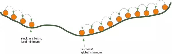
Continuing in this manner, you eventually reach a point where further descent is no longer possible. Each direction goes upwards. You may have reached the deepest level. Really the deppest level, i.e. sea level? You may find yourself in a local minimum instead of the global minimum, you are stuck in a basin. Starting from the right side of our illustration leads to the desired outcome, but beginning from the left side could trap you in a local minimum.
If you start at the position on the right side of our image, everything works out fine, but from the leftside, you will be stuck in a local minimum.
Live Python training

Enjoying this page? We offer live Python training courses covering the content of this site.
See our Python training courses
Backpropagation in Detail
Now, we have to go into the details, i.e. the mathematics.
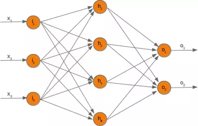
We will start with the simpler case. We look at a linear network. Linear neural networks are networks where the output signal is created by summing up all the weighted input signals. No activation function will be applied to this sum, which is the reason for the linearity.
The will use the following simple network.
When training a neural network, we have samples with corresponding labels. For each output value $ o_i $, there's a corresponding label $ t_i $, which represents the desired or target value. The error $ e_i $ for each output is calculated as the difference between the target and the actual output:
To quantify the overall performance of the network, we use a squared error function, which sums the squared differences between the target and actual outputs:
This function is preferred because it ensures all errors are positive and penalizes larger errors more heavily, facilitating faster convergence during training.
We aim to elucidate the process of error backpropagation through an illustrative example using specific values. However, our focus will be solely on a single node for now:
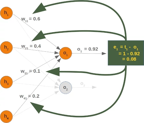
We will have a look at the output value $o_1$, which is depending on the values $w_{11}$, $w_{12}$, $w_{13}$ and $w_{14}$. Let's assume the calculated value ($o_1$) is 0.92 and the desired value ($t_1$) is 1. In this case the error is
In response to this error, adjustments must be made to the weights connected to the output of the hidden layer. For the sake of convenience, we will simply use "$w$" instead of "$wh$". With four weights in consideration, a uniform distribution of the error across them might seem plausible. However, a more effective approach is to distribute the error proportionally based on the weight values. The significance of a weight in relation to others determines its responsibility for the error. Thus, the fraction of the error $e_1$ attributed to $w_{11}$ can be calculated as:
For instance, in our example:
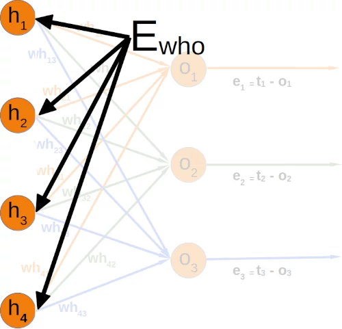
The total error in the weight matrix between the hidden and output layers (referred to as 'who' in our previous chapter) is represented as:
# example who:
import numpy as np


who = np.array([[0.6, 0.5, 0.06],
                [0.3, 0.2, 0.8],
                [0.2, 0.1, 0.7],
                [0.12, 0.7, 0.54]])

e = np.array([0.1, 0.2, 0.3])

who * e
OUTPUT:
array([[0.06 , 0.1  , 0.018],
       [0.03 , 0.04 , 0.24 ],
       [0.02 , 0.02 , 0.21 ],
       [0.012, 0.14 , 0.162]])
You can see that the denominator in the left matrix is always the same for each column. It functions like a scaling factor. We can drop it so that the calculation gets a lot simpler:
If you compare the matrix on the right side with the 'who' matrix of our chapter Neuronal Network Using Python and Numpy, you will notice that it is the transpose of 'who'.
So, this has been the easy part for linear neural networks. We haven't taken into account the activation function until now.
We want to calculate the error in a network with an activation function, i.e. a non-linear network. The derivation of the error function describes the slope. As we mentioned in the beginning of the this chapter, we want to descend. The derivation describes how the error $E$ changes as the weight $w_{jk}$ changes:
The error function E over all the output nodes $o_i$ ($i = 1, ... n$) where $n$ is the total number of output nodes:
Now, we can insert this in our derivation:
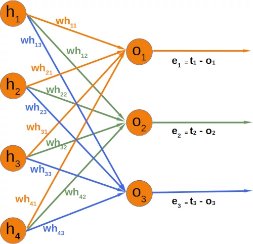
If you have a look at our example network, you will see that an output node $o_k$ only depends on the input signals created with the weights $w_{ik}$ with $i = 1, \ldots m$ and $m$ the number of hidden nodes.
The following diagram further illuminates this:
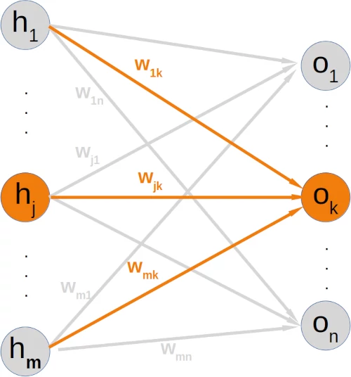
This means that we can calculate the error for every output node independently of each other. This means that we can remove all expressions $t_i - o_i$ with $i \neq k$ from our summation. So the calculation of the error for a node k looks a lot simpler now:
The target value $t_k$ is a constant, because it is not depending on any input signals or weights. We can apply the chain rule for the differentiation of the previous term to simplify things:
In the previous chapter of our tutorial, we used the sigmoid function as the activation function:
The output node $o_k$ is calculated by applying the sigmoid function to the sum of the weighted input signals. This means that we can further transform our derivative term by replacing $o_k$ by this function:
equivalent to
replacing $o_k$ by its calculation:
where $m$ is the number of hidden nodes.
The sigmoid function is easy to differentiate:
The complete differentiation looks like this now:
The last part has to be differentiated with respect to $w_{jk}$. This means that the derivation of all the products will be 0 except the the term $ w_{jk}h_j)$ which has the derivative $h_j$ with respect to $w_{jk}$:
substituting $\sigma(\sum_{i=1}^{m} w_{ik}h_i)$ by $o_k$:
This is what we need to implement the method 'train' of our NeuralNetwork class in the following chapter.
Live Python training
Enjoying this page? We offer live Python training courses covering the content of this site.
Upcoming online Courses
See our Python training courses