7. Train and Test Sets by Splitting Learn and Test Data
By Bernd Klein. Last modified: 07 Mar 2024.
Learn, Test and Evaluation Data
You have your data ready and you are eager to start training the classifier? But be careful: When your classifier will be finished, you will need some test data to evaluate your classifier. If you evaluate your classifier with the data used for learning, you may see surprisingly good results. What we actually want to test is the performance of classifying on unknown data.
For this purpose, we need to split our data into two parts:
- A training set with which the learning algorithm adapts or learns the model
- A test set to evaluate the generalization performance of the model
When you consider how machine learning normally works, the idea of a split between learning and test data makes sense. Really existing systems train on existing data and if other new data (from customers, sensors or other sources) comes in, the trained classifier has to predict or classify this new data. We can simulate this during training with a training and test data set - the test data is a simulation of "future data" that will go into the system during production.
In this chapter of our Python Machine Learning Tutorial, we will learn how to do the splitting with plain Python.
We will see also that doing it manually is not necessary, because the train_test_split function from the model_selection module can do it for us.
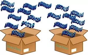
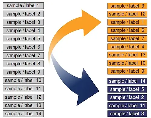
If the dataset is sorted by label, we will have to shuffle it before splitting.
We separated the dataset into a learn (a.k.a. training) dataset and a test dataset. Best practice is to split it into a learn, test and an evaluation dataset.
We will train our model (classifier) step by step and each time the result needs to be tested. If we just have a test dataset. The results of the testing might get into the model. So we will use an evaluation dataset for the complete learning phase. When our classifier is finished, we will check it with the test dataset, which it has not "seen" before!
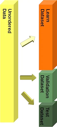
Yet, during our tutorial, we will only use splitings into learn and test datasets.
Live Python training

Enjoying this page? We offer live Python training courses covering the content of this site.
Splitting Example: Iris Data Set
We will demonstrate the previously discussed topics with the Iris Dataset.
The 150 data sets of the Iris data set are sorted, i.e. the first 50 data correspond to the first flower class (0 = Setosa), the next 50 to the second flower class (1 = Versicolor) and the remaining data correspond to the last class (2 = Virginica).
If we were to split our data in the ratio 2/3 (learning set) and 1/3 (test set), the learning set would contain all the flowers of the first two classes and the test set all the flowers of the third flower class. The classifier could only learn two classes and the third class would be completely unknown. So we urgently need to mix the data.
Assuming all samples are independent of each other, we want to shuffle the data set randomly before we split the data set as shown above.
In the following we split the data manually:
import numpy as np
from sklearn.datasets import load_iris
iris = load_iris()
Looking at the labels of iris.target shows us that the data is sorted.
iris.target
OUTPUT:
array([0, 0, 0, 0, 0, 0, 0, 0, 0, 0, 0, 0, 0, 0, 0, 0, 0, 0, 0, 0, 0, 0,
       0, 0, 0, 0, 0, 0, 0, 0, 0, 0, 0, 0, 0, 0, 0, 0, 0, 0, 0, 0, 0, 0,
       0, 0, 0, 0, 0, 0, 1, 1, 1, 1, 1, 1, 1, 1, 1, 1, 1, 1, 1, 1, 1, 1,
       1, 1, 1, 1, 1, 1, 1, 1, 1, 1, 1, 1, 1, 1, 1, 1, 1, 1, 1, 1, 1, 1,
       1, 1, 1, 1, 1, 1, 1, 1, 1, 1, 1, 1, 2, 2, 2, 2, 2, 2, 2, 2, 2, 2,
       2, 2, 2, 2, 2, 2, 2, 2, 2, 2, 2, 2, 2, 2, 2, 2, 2, 2, 2, 2, 2, 2,
       2, 2, 2, 2, 2, 2, 2, 2, 2, 2, 2, 2, 2, 2, 2, 2, 2, 2])
The first thing we have to do is rearrange the data so that it is not sorted anymore. For this purpose, we will use the permutation function of the random submodul of Numpy:
indices = np.random.permutation(len(iris.data))
indices
OUTPUT:
array([145, 140,  55,  83,  50,  42,  66,  12,  52,  39, 114,  80, 108,
        38, 119,  30, 112, 142, 101, 144,  33,   5,  40,  87,  29,  24,
        16, 130, 128,  89,  23,  60,  96,  36,  82,  56, 136,  58, 106,
        70, 110,  15,   2,  97, 115, 133,  88,  61, 139,  54,  10, 132,
        47,  71,   6,  41,  85,  45,  67,   7, 118,  95,  63,   3, 127,
       134,  13, 113,  46, 137,  90,  94, 121,  21,  98,  99,  34,  76,
        35, 105,  44,  48,  43, 143,  92,  20,   1,  32, 129,  91,  84,
       104,  59,  73,   4, 138,  68,   9, 148,  49,  78, 122,  11,  19,
       131,  65,   0,  77,  26, 147,  57, 125,  74, 100, 126,  25,  86,
       120,  18,  75,  14,  53,  37, 135, 103,   8, 117, 124, 123, 141,
       111,  72,  62,  69, 109,  31, 149, 102,  64,  22, 107,  79,  28,
        81, 146, 116,  51,  27,  17,  93])
n_test_samples = 12
learnset_data = iris.data[indices[:-n_test_samples]]
learnset_labels = iris.target[indices[:-n_test_samples]]
testset_data = iris.data[indices[-n_test_samples:]]
testset_labels = iris.target[indices[-n_test_samples:]]
print(learnset_data[:4], learnset_labels[:4])
print(testset_data[:4], testset_labels[:4])
OUTPUT:
[[6.7 3.  5.2 2.3]
 [6.7 3.1 5.6 2.4]
 [5.7 2.8 4.5 1.3]
 [6.  2.7 5.1 1.6]] [2 2 1 1]
[[5.6 2.9 3.6 1.3]
 [4.6 3.6 1.  0.2]
 [7.3 2.9 6.3 1.8]
 [5.7 2.6 3.5 1. ]] [1 0 2 1]
Splits with Sklearn
Even though it was not difficult to split the data manually into a learn (train) and an evaluation (test) set, we don't have to do the splitting manually as shown above. Since this is often required in machine learning, scikit-learn has a predefined function for dividing data into training and test sets.
We will demonstrate this below. We will use 80% of the data as training and 20% as test data. We could just as well have taken 70% and 30%, because there are no hard and fast rules. The most important thing is that you rate your system fairly based on data it * did not * see during exercise! In addition, there must be enough data in both data sets.
from sklearn.datasets import load_iris
from sklearn.model_selection import train_test_split
iris = load_iris()
data, labels = iris.data, iris.target

res = train_test_split(data, labels,
                       train_size=0.8,
                       test_size=0.2,
                       random_state=42)
train_data, test_data, train_labels, test_labels = res

n = 7
print(f"The first {n} data sets:")
print(test_data[:7])
print(f"The corresponding {n} labels:")
print(test_labels[:7])
OUTPUT:
The first 7 data sets:
[[6.1 2.8 4.7 1.2]
 [5.7 3.8 1.7 0.3]
 [7.7 2.6 6.9 2.3]
 [6.  2.9 4.5 1.5]
 [6.8 2.8 4.8 1.4]
 [5.4 3.4 1.5 0.4]
 [5.6 2.9 3.6 1.3]]
The corresponding 7 labels:
[1 0 2 1 1 0 1]
Let's proceed to visualize our training and testing datasets. In our plot, green and blue points will denote the training data, whereas light green and light blue points will symbolize the testing data.
import matplotlib.pyplot as plt

fig, ax = plt.subplots()
# plotting learn data
colours = ('green', 'blue')
for n_class in range(2):
    ax.scatter(train_data[train_labels==n_class][:, 0],
               train_data[train_labels==n_class][:, 1],
               c=colours[n_class], s=40, label=str(n_class))


# plotting test data
colours = ('lightgreen', 'lightblue')
for n_class in range(2):
    ax.scatter(test_data[test_labels==n_class][:, 0],
               test_data[test_labels==n_class][:, 1],
               c=colours[n_class], s=40, label=str(n_class))

ax.plot()
OUTPUT:
[]

The followong code improves readability and modularity by creating a separate function for plotting the data. It also adds a legend to the plot for better interpretation of the classes:
import matplotlib.pyplot as plt

# Define function for scatter plot
def plot_data(data, labels, ax, colours, label):
    for n_class, colour in enumerate(colours):
        ax.scatter(data[labels == n_class][:, 0],
                   data[labels == n_class][:, 1],
                   c=colour, s=40, label=label.format(n_class))

# Create figure and axis objects
fig, ax = plt.subplots()

# Plot training data
train_colours = ['green', 'blue']
plot_data(train_data, train_labels, ax, train_colours, label="Training Class {}")

# Plot testing data
test_colours = ['lightgreen', 'lightblue']
plot_data(test_data, test_labels, ax, test_colours, label="Testing Class {}")

# Add legend
ax.legend()

# Show plot
plt.show()

Live Python training
Enjoying this page? We offer live Python training courses covering the content of this site.
Upcoming online Courses
Stratified random sample
Especially with relatively small amounts of data, it is better to stratify the division. Stratification means that we keep the original class proportion of the data set in the test and training sets. We calculate the class proportions of the previous split in percent using the following code. To calculate the number of occurrences of each class, we use the numpy function 'bincount'. It counts the number of occurrences of each value in the array of non-negative integers passed as an argument.
import numpy as np
print('All:', np.bincount(labels) / float(len(labels)) * 100.0)
print('Training:', np.bincount(train_labels) / float(len(train_labels)) * 100.0)
print('Test:', np.bincount(test_labels) / float(len(test_labels)) * 100.0)
OUTPUT:
All: [33.33333333 33.33333333 33.33333333]
Training: [33.33333333 34.16666667 32.5       ]
Test: [33.33333333 30.         36.66666667]
To stratify the division, we can pass the label array as an additional argument to the train_test_split function:
from sklearn.datasets import load_iris
from sklearn.model_selection import train_test_split
iris = load_iris()
data, labels = iris.data, iris.target

res = train_test_split(data, labels,
                       train_size=0.8,
                       test_size=0.2,
                       random_state=42,
                       stratify=labels)
train_data, test_data, train_labels, test_labels = res

print('All:', np.bincount(labels) / float(len(labels)) * 100.0)
print('Training:', np.bincount(train_labels) / float(len(train_labels)) * 100.0)
print('Test:', np.bincount(test_labels) / float(len(test_labels)) * 100.0)
OUTPUT:
All: [33.33333333 33.33333333 33.33333333]
Training: [33.33333333 33.33333333 33.33333333]
Test: [33.33333333 33.33333333 33.33333333]
This was a stupid example to test the stratified random sample, because the Iris data set has the same proportions, i.e. each class 50 elements.
We will work now with the file strange_flowers.txt of the directory data. This data set is created in the chapter Generate Datasets in Python
The classes in this dataset have different numbers of items. First we load the data:
content = np.loadtxt("data/strange_flowers.txt", delimiter=" ")
data = content[:, :-1]    # cut of the target column
labels = content[:, -1]
labels.dtype
labels.shape
OUTPUT:
(795,)
res = train_test_split(data, labels,
                       train_size=0.8,
                       test_size=0.2,
                       random_state=42,
                       stratify=labels)
train_data, test_data, train_labels, test_labels = res

# np.bincount expects non negative integers:
print('All:', np.bincount(labels.astype(int))  / float(len(labels)) * 100.0)
print('Training:', np.bincount(train_labels.astype(int)) / float(len(train_labels)) * 100.0)
print('Test:', np.bincount(test_labels.astype(int)) / float(len(test_labels)) * 100.0)
OUTPUT:
All: [ 0.         23.89937107 25.78616352 28.93081761 21.3836478 ]
Training: [ 0.         23.89937107 25.78616352 28.93081761 21.3836478 ]
Test: [ 0.         23.89937107 25.78616352 28.93081761 21.3836478 ]
Exercises
Exercise 1
In this exercise, you will practice performing a train-test split on the Wine dataset from scikit-learn. The Wine dataset contains the results of a chemical analysis of three different sorts of wine. Each sample is categorized into one of three classes. Your task is to split this dataset into training and testing sets with a 70-30 ratio, where 70% of the data will be used for training and 30% for testing.
Print the shapes of the created datasets.
Live Python training
Enjoying this page? We offer live Python training courses covering the content of this site.
Solutions
Solution to Exercise 1
from sklearn.datasets import load_wine
from sklearn.model_selection import train_test_split

# Load the Wine dataset
wine = load_wine()

X = wine.data
y = wine.target

# Perform train-test split with 70% training and 30% testing
X_train, X_test, y_train, y_test = train_test_split(X, y, test_size=0.3, random_state=42)

# Print the shapes of the resulting train and test sets
print("X_train shape:", X_train.shape)
print("X_test shape:", X_test.shape)
print("y_train shape:", y_train.shape)
print("y_test shape:", y_test.shape)
OUTPUT:
X_train shape: (124, 13)
X_test shape: (54, 13)
y_train shape: (124,)
y_test shape: (54,)
Live Python training
Enjoying this page? We offer live Python training courses covering the content of this site.
Upcoming online Courses