5. Available Data Sets in Sklearn
By Bernd Klein. Last modified: 19 Apr 2024.

Scikit-learn makes available a host of datasets for testing learning algorithms. They come in three flavors:
- Packaged Data: these small datasets are packaged with the scikit-learn installation,
and can be downloaded using the tools in
sklearn.datasets.load_* - Downloadable Data: these larger datasets are available for download, and scikit-learn
includes tools which streamline this process. These tools can be found in
sklearn.datasets.fetch_* - Generated Data: there are several datasets which are generated from models based on a
random seed. These are available in the
sklearn.datasets.make_*
You can explore the available dataset loaders, fetchers, and generators using IPython's
tab-completion functionality. After importing the datasets submodule from sklearn,
type
datasets.load_<TAB>
or
datasets.fetch_<TAB>
or
datasets.make_<TAB>
to see a list of available functions.
Structure of Data and Labels
Data in scikit-learn is in most cases saved as two-dimensional Numpy arrays with the shape (n, m). Many algorithms also accept scipy.sparse matrices of the same shape.
- n: (n_samples) The number of samples: each sample is an item to process (e.g. classify). A sample can be a document, a picture, a sound, a video, an astronomical object, a row in database or CSV file, or whatever you can describe with a fixed set of quantitative traits.
- m: (m_features) The number of features or distinct traits that can be used to describe each item in a quantitative manner. Features are generally real-valued, but may be Boolean or discrete-valued in some cases.
from sklearn import datasets
Be warned: many of these datasets are quite large, and can take a long time to download!
Live Python training

Enjoying this page? We offer live Python training courses covering the content of this site.
See our Python training courses
Loading Digits Data
We will have a closer look at one of these datasets. We look at the digits data set. We will load it first:
from sklearn.datasets import load_digits
digits = load_digits()
Again, we can get an overview of the available attributes by looking at the "keys":
digits.keys()
OUTPUT:
dict_keys(['data', 'target', 'frame', 'feature_names', 'target_names', 'images', 'DESCR'])
Let's have a look at the number of items and features:
n_samples, n_features = digits.data.shape
print((n_samples, n_features))
OUTPUT:
(1797, 64)
print(digits.data[0])
print(digits.target)
OUTPUT:
[ 0.  0.  5. 13.  9.  1.  0.  0.  0.  0. 13. 15. 10. 15.  5.  0.  0.  3.
 15.  2.  0. 11.  8.  0.  0.  4. 12.  0.  0.  8.  8.  0.  0.  5.  8.  0.
  0.  9.  8.  0.  0.  4. 11.  0.  1. 12.  7.  0.  0.  2. 14.  5. 10. 12.
  0.  0.  0.  0.  6. 13. 10.  0.  0.  0.]
[0 1 2 ... 8 9 8]
The data is also available at digits.images. This is the raw data of the images in the form of 8 lines and 8 columns.
With "data" an image corresponds to a one-dimensional Numpy array with the length 64, and "images" representation contains 2-dimensional numpy arrays with the shape (8, 8)
print("Shape of an item: ", digits.data[0].shape)
print("Data type of an item: ", type(digits.data[0]))
print("Shape of an item: ", digits.images[0].shape)
print("Data tpye of an item: ", type(digits.images[0]))
OUTPUT:
Shape of an item:  (64,)
Data type of an item:  <class 'numpy.ndarray'>
Shape of an item:  (8, 8)
Data tpye of an item:  <class 'numpy.ndarray'>
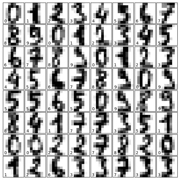
Let's visualize the data. It's little bit more involved than the simple scatter-plot we used above, but we can do it rather quickly.
# visualisation of the digits data set
import matplotlib.pyplot as plt
# set up the figure
fig = plt.figure(figsize=(6, 6))  # figure size in inches
fig.subplots_adjust(left=0, right=1, bottom=0, top=1, hspace=0.05, wspace=0.05)

# plot the digits: each image is 8x8 pixels
for i in range(64):
    ax = fig.add_subplot(8, 8, i + 1, xticks=[], yticks=[])
    ax.imshow(digits.images[i], cmap=plt.cm.binary, interpolation='nearest')

    # label the image with the target value
    ax.text(0, 7, str(digits.target[i]))
Exercises
Exercise 1
sklearn contains a "wine data set".
- Find and load this data set
- Can you find a description?
- What are the names of the classes?
- What are the features?
- Where is the data and the labeled data?
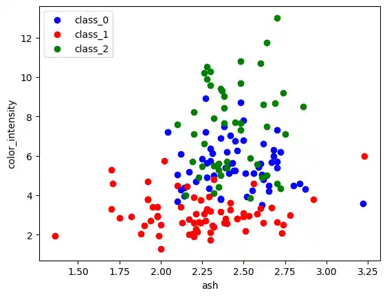
Exercise 2:
Create a scatter plot of the features ash and color_intensity of the wine data set.
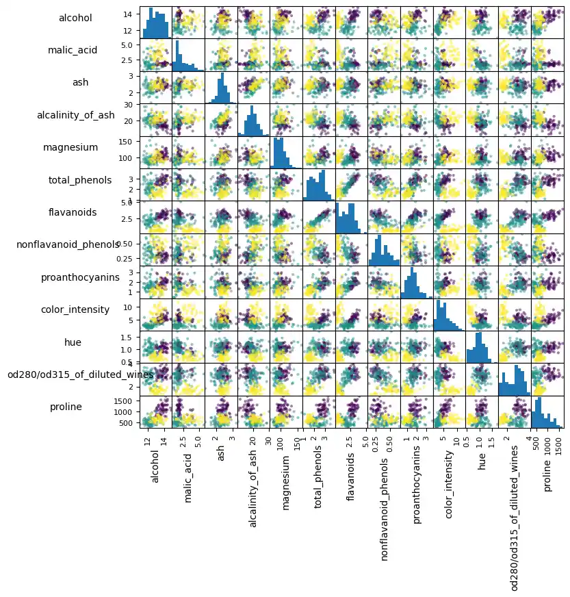
Exercise 3:
Create a scatter matrix of the features of the wine dataset.
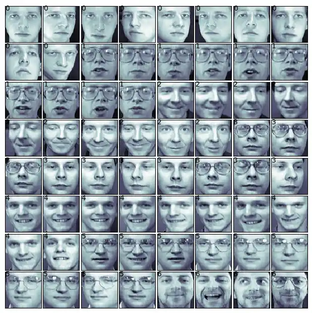
Exercise 4:
Fetch the Olivetti faces dataset and visualize the faces.
Live Python training
Enjoying this page? We offer live Python training courses covering the content of this site.
Upcoming online Courses
See our Python training courses
Solutions
Solution to Exercise 1
Loading the "wine data set":
from sklearn import datasets

wine = datasets.load_wine()
The description can be accessed via "DESCR":
print(wine.DESCR)
OUTPUT:
.. _wine_dataset:

Wine recognition dataset
------------------------

**Data Set Characteristics:**

    :Number of Instances: 178
    :Number of Attributes: 13 numeric, predictive attributes and the class
    :Attribute Information:
 		- Alcohol
 		- Malic acid
 		- Ash
		- Alcalinity of ash
 		- Magnesium
		- Total phenols
 		- Flavanoids
 		- Nonflavanoid phenols
 		- Proanthocyanins
		- Color intensity
 		- Hue
 		- OD280/OD315 of diluted wines
 		- Proline

    - class:
            - class_0
            - class_1
            - class_2

    :Summary Statistics:

    ============================= ==== ===== ======= =====
                                   Min   Max   Mean     SD
    ============================= ==== ===== ======= =====
    Alcohol:                      11.0  14.8    13.0   0.8
    Malic Acid:                   0.74  5.80    2.34  1.12
    Ash:                          1.36  3.23    2.36  0.27
    Alcalinity of Ash:            10.6  30.0    19.5   3.3
    Magnesium:                    70.0 162.0    99.7  14.3
    Total Phenols:                0.98  3.88    2.29  0.63
    Flavanoids:                   0.34  5.08    2.03  1.00
    Nonflavanoid Phenols:         0.13  0.66    0.36  0.12
    Proanthocyanins:              0.41  3.58    1.59  0.57
    Colour Intensity:              1.3  13.0     5.1   2.3
    Hue:                          0.48  1.71    0.96  0.23
    OD280/OD315 of diluted wines: 1.27  4.00    2.61  0.71
    Proline:                       278  1680     746   315
    ============================= ==== ===== ======= =====

    :Missing Attribute Values: None
    :Class Distribution: class_0 (59), class_1 (71), class_2 (48)
    :Creator: R.A. Fisher
    :Donor: Michael Marshall (MARSHALL%[email protected])
    :Date: July, 1988

This is a copy of UCI ML Wine recognition datasets.
https://archive.ics.uci.edu/ml/machine-learning-databases/wine/wine.data

The data is the results of a chemical analysis of wines grown in the same
region in Italy by three different cultivators. There are thirteen different
measurements taken for different constituents found in the three types of
wine.

Original Owners:

Forina, M. et al, PARVUS -
An Extendible Package for Data Exploration, Classification and Correlation.
Institute of Pharmaceutical and Food Analysis and Technologies,
Via Brigata Salerno, 16147 Genoa, Italy.

Citation:

Lichman, M. (2013). UCI Machine Learning Repository
[https://archive.ics.uci.edu/ml]. Irvine, CA: University of California,
School of Information and Computer Science.

|details-start|
**References**
|details-split|

(1) S. Aeberhard, D. Coomans and O. de Vel,
Comparison of Classifiers in High Dimensional Settings,
Tech. Rep. no. 92-02, (1992), Dept. of Computer Science and Dept. of
Mathematics and Statistics, James Cook University of North Queensland.
(Also submitted to Technometrics).

The data was used with many others for comparing various
classifiers. The classes are separable, though only RDA
has achieved 100% correct classification.
(RDA : 100%, QDA 99.4%, LDA 98.9%, 1NN 96.1% (z-transformed data))
(All results using the leave-one-out technique)

(2) S. Aeberhard, D. Coomans and O. de Vel,
"THE CLASSIFICATION PERFORMANCE OF RDA"
Tech. Rep. no. 92-01, (1992), Dept. of Computer Science and Dept. of
Mathematics and Statistics, James Cook University of North Queensland.
(Also submitted to Journal of Chemometrics).

|details-end|
The names of the classes and the features can be retrieved like this:
print(wine.target_names)
print(wine.feature_names)
OUTPUT:
['class_0' 'class_1' 'class_2']
['alcohol', 'malic_acid', 'ash', 'alcalinity_of_ash', 'magnesium', 'total_phenols', 'flavanoids', 'nonflavanoid_phenols', 'proanthocyanins', 'color_intensity', 'hue', 'od280/od315_of_diluted_wines', 'proline']
data = wine.data
labelled_data = wine.target
Solution to Exercise 2:
from sklearn import datasets
import matplotlib.pyplot as plt

wine = datasets.load_wine()

features = 'ash', 'color_intensity'
features_index = [wine.feature_names.index(features[0]),
                  wine.feature_names.index(features[1])]


colors = ['blue', 'red', 'green']

for label, color in zip(range(len(wine.target_names)), colors):
    plt.scatter(wine.data[wine.target==label, features_index[0]],
                wine.data[wine.target==label, features_index[1]],
                label=wine.target_names[label],
                c=color)

plt.xlabel(features[0])
plt.ylabel(features[1])
plt.legend(loc='upper left')
plt.show() # wine dataset scatter plot
Solution to Exercise 3:
# scatter matrix of wine data set
import pandas as pd
from sklearn import datasets

wine = datasets.load_wine()
def rotate_labels(df, axes):
    """ changing the rotation of the label output,
    y labels horizontal and x labels vertical """
    n = len(df.columns)
    for x in range(n):
        for y in range(n):
            # to get the axis of subplots
            ax = axs[x, y]
            # to make x axis name vertical
            ax.xaxis.label.set_rotation(90)
            # to make y axis name horizontal
            ax.yaxis.label.set_rotation(0)
            # to make sure y axis names are outside the plot area
            ax.yaxis.labelpad = 50

wine_df = pd.DataFrame(wine.data, columns=wine.feature_names)
axs = pd.plotting.scatter_matrix(wine_df,
                                 c=wine.target,
                                 figsize=(8, 8),
                                );

rotate_labels(wine_df, axs)
Solution to Exercise 4
from sklearn.datasets import fetch_olivetti_faces
# fetch the faces data
faces = fetch_olivetti_faces()
OUTPUT:
downloading Olivetti faces from https://ndownloader.figshare.com/files/5976027 to /home/bernd/scikit_learn_data
faces.keys()
OUTPUT:
dict_keys(['data', 'images', 'target', 'DESCR'])
n_samples, n_features = faces.data.shape
print((n_samples, n_features))
OUTPUT:
(400, 4096)
import numpy as np
np.sqrt(4096)
OUTPUT:
64.0
faces.images.shape
OUTPUT:
(400, 64, 64)
import numpy as np
print(np.all(faces.images.reshape((400, 4096)) == faces.data))
OUTPUT:
True
# visualisation of faces dataset
fig = plt.figure(figsize=(6, 6))  # figure size in inches
fig.subplots_adjust(left=0, right=1, bottom=0, top=1, hspace=0.05, wspace=0.05)

# plot the digits: each image is 8x8 pixels
for i in range(64):
    ax = fig.add_subplot(8, 8, i + 1, xticks=[], yticks=[])
    ax.imshow(faces.images[i], cmap=plt.cm.bone, interpolation='nearest')

    # label the image with the target value
    ax.text(0, 7, str(faces.target[i]))
Further Datasets
sklearn has many more datasets available. If you still need more, you will find more on this nice List of datasets for machine-learning research at Wikipedia.
Live Python training
Enjoying this page? We offer live Python training courses covering the content of this site.
Upcoming online Courses
See our Python training courses