8. k-Nearest Neighbor Classifier in Python
By Bernd Klein. Last modified: 19 Apr 2024.

"Show me who your friends are and I’ll tell you who you are?"
The concept of the k-nearest neighbor classifier can hardly be simpler described. This is an old saying, which can be found in many languages and many cultures. It's also metnioned in other words in the Bible: "He who walks with wise men will be wise, but the companion of fools will suffer harm" (Proverbs 13:20 )
This means that the concept of the k-nearest neighbor classifier is part of our everyday life and judging: Imagine you meet a group of people, they are all very young, stylish and sportive. They talk about there friend Ben, who isn't with them. So, what is your imagination of Ben? Right, you imagine him as being yong, stylish and sportive as well.
If you learn that Ben lives in a neighborhood where people vote conservative and that the average income is above 200000 dollars a year? Both his neighbors make even more than 300,000 dollars per year? What do you think of Ben? Most probably, you do not consider him to be an underdog and you may suspect him to be a conservative as well?
The principle behind nearest neighbor classification consists in finding a predefined number, i.e. the 'k' - of training samples closest in distance to a new sample, which has to be classified. The label of the new sample will be defined from these neighbors. k-nearest neighbor classifiers have a fixed user defined constant for the number of neighbors which have to be determined. There are also radius-based neighbor learning algorithms, which have a varying number of neighbors based on the local density of points, all the samples inside of a fixed radius. The distance can, in general, be any metric measure: standard Euclidean distance is the most common choice. Neighbors-based methods are known as non-generalizing machine learning methods, since they simply "remember" all of its training data. Classification can be computed by a majority vote of the nearest neighbors of the unknown sample.
The k-NN algorithm is among the simplest of all machine learning algorithms, but despite its simplicity, it has been quite successful in a large number of classification and regression problems, for example character recognition or image analysis.
Now let's get a little bit more mathematically:
As explained in the chapter Data Preparation, we need labeled learning and test data. In contrast to other classifiers, however, the pure nearest-neighbor classifiers do not do any learning, but the so-called learning set $LS$ is a basic component of the classifier. The k-Nearest-Neighbor Classifier (kNN) works directly on the learned samples, instead of creating rules compared to other classification methods.
Nearest Neighbor Algorithm:
Given a set of categories $C = \{c_1, c_2, ... c_m\}$, also called classes, e.g. {"male", "female"}. There is also a learnset $LS$ consisting of labelled instances:
As it makes no sense to have less lebelled items than categories, we can postulate that
$n > m$ and in most cases even $n \ggg m$ (n much greater than m.)
The task of classification consists in assigning a category or class $c$ to an arbitrary instance $o$.
For this, we have to differentiate between two cases:
- Case 1:
The instance $o$ is an element of $LS$, i.e. there is a tupel $(o, c) \in LS$
In this case, we will use the class $c$ as the classification result. - Case 2:
We assume now that $o$ is not in $LS$, or to be precise:
$\forall c \in C, (o, c) \not\in LS$
$o$ is compared with all the instances of $LS$. A distance metric $d$ is used for the comparisons.
We determine the $k$ closest neighbors of $o$, i.e. the items with the smallest distances.
$k$ is a user defined constant and a positive integer, which is usually small.
The number $k$ is typically chosen as the square root of $LS$, the total number of points in the training data set.
To determine the $k$ nearest neighbors we reorder $LS$ in the following way:
$(o_{i_1}, c_{o_{i_1}}), (o_{i_2}, c_{o_{i_2}}), \cdots (o_{i_n}, c_{o_{i_n}})$
so that $d(o_{i_j}, o) \leq d(o_{i_{j+1}}, o)$ is true for all $1 \leq j \leq {n-1}$
The set of k-nearest neighbors $N_k$ consists of the first $k$ elements of this ordering, i.e.
$N_k = \{ (o_{i_1}, c_{o_{i_1}}), (o_{i_2}, c_{o_{i_2}}), \cdots (o_{i_k}, c_{o_{i_k}}) \}$
The most common class in this set of nearest neighbors $N_k$ will be assigned to the instance $o$. If there is no unique most common class, we take an arbitrary one of these.
There is no general way to define an optimal value for 'k'. This value depends on the data. As a general rule we can say that increasing 'k' reduces the noise but on the other hand makes the boundaries less distinct.
The algorithm for the k-nearest neighbor classifier is among the simplest of all machine learning algorithms. k-NN is a type of instance-based learning, or lazy learning. In machine learning, lazy learning is understood to be a learning method in which generalization of the training data is delayed until a query is made to the system. On the other hand, we have eager learning, where the system usually generalizes the training data before receiving queries. In other words: The function is only approximated locally and all the computations are performed, when the actual classification is being performed.
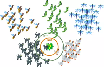
The following picture shows in a simple way how the nearest neighbor classifier works. The puzzle piece is unknown. To find out which animal it might be we have to find the neighbors. If k=1, the only neighbor is a cat and we assume in this case that the puzzle piece should be a cat as well. If k=4, the nearest neighbors contain one chicken and three cats. In this case again, it will be save to assume that our object in question should be a cat.
k-nearest-neighbor from Scratch
Preparing the Dataset
Before we actually start with writing a nearest neighbor classifier, we need to think about the data, i.e. the learnset and the testset. We will use the "iris" dataset provided by the datasets of the sklearn module.
The data set consists of 50 samples from each of three species of Iris
- Iris setosa,
- Iris virginica and
- Iris versicolor.
Four features were measured from each sample: the length and the width of the sepals and petals, in centimetres.
import numpy as np
from sklearn import datasets

iris = datasets.load_iris()
data = iris.data
labels = iris.target

for i in [0, 79, 99, 121]:
    print(f"index: {i:3}, features: {data[i]}, label: {labels[i]}")
OUTPUT:
index:   0, features: [5.1 3.5 1.4 0.2], label: 0
index:  79, features: [5.7 2.6 3.5 1. ], label: 1
index:  99, features: [5.7 2.8 4.1 1.3], label: 1
index: 121, features: [5.6 2.8 4.9 2. ], label: 2
We create a learnset from the sets above. We use permutation from np.random to split the data randomly.
# seeding is only necessary for the website
#so that the values are always equal:
np.random.seed(42)
indices = np.random.permutation(len(data))

n_test_samples = 12     # number of test samples
learn_data = data[indices[:-n_test_samples]]
learn_labels = labels[indices[:-n_test_samples]]
test_data = data[indices[-n_test_samples:]]
test_labels = labels[indices[-n_test_samples:]]

print("The first samples of our learn set:")
print(f"{'index':7s}{'data':20s}{'label':3s}")
for i in range(5):
    print(f"{i:4d}   {learn_data[i]}   {learn_labels[i]:3}")

print("The first samples of our test set:")
print(f"{'index':7s}{'data':20s}{'label':3s}")
for i in range(5):
    print(f"{i:4d}   {learn_data[i]}   {learn_labels[i]:3}")
OUTPUT:
The first samples of our learn set:
index  data                label
   0   [6.1 2.8 4.7 1.2]     1
   1   [5.7 3.8 1.7 0.3]     0
   2   [7.7 2.6 6.9 2.3]     2
   3   [6.  2.9 4.5 1.5]     1
   4   [6.8 2.8 4.8 1.4]     1
The first samples of our test set:
index  data                label
   0   [6.1 2.8 4.7 1.2]     1
   1   [5.7 3.8 1.7 0.3]     0
   2   [7.7 2.6 6.9 2.3]     2
   3   [6.  2.9 4.5 1.5]     1
   4   [6.8 2.8 4.8 1.4]     1
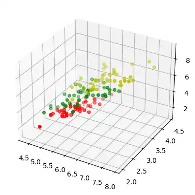
The following code is only necessary to visualize the data of our learnset. Our data consists of four values per iris item, so we will reduce the data to three values by summing up the third and fourth value. This way, we are capable of depicting the data in 3-dimensional space:
#%matplotlib widget

import matplotlib.pyplot as plt
from mpl_toolkits.mplot3d import Axes3D

colours = ("r", "b")
X = []
for iclass in range(3):
    X.append([[], [], []])
    for i in range(len(learn_data)):
        if learn_labels[i] == iclass:
            X[iclass][0].append(learn_data[i][0])
            X[iclass][1].append(learn_data[i][1])
            X[iclass][2].append(sum(learn_data[i][2:]))

colours = ("r", "g", "y")

fig = plt.figure()
ax = fig.add_subplot(111, projection='3d')

for iclass in range(3):
       ax.scatter(X[iclass][0],
                  X[iclass][1],
                  X[iclass][2],
                  c=colours[iclass])
plt.show()
Distance metrics
We have already mentioned in detail, we calculate the distances between the points of the sample and the object to be classified. To calculate these distances we need a distance function.
In n-dimensional vector rooms, one usually uses one of the following three distance metrics:
-
Euclidean Distance
The Euclidean distance between two points
xandyin either the plane or 3-dimensional space measures the length of a line segment connecting these two points. It can be calculated from the Cartesian coordinates of the points using the Pythagorean theorem, therefore it is also occasionally being called the Pythagorean distance. The general formula is$$d(x, y) = \sqrt{\sum_{i=1}^{n} (x_i -y_i)^2}$$ -
Manhattan Distance
It is defined as the sum of the absolute values of the differences between the coordinates of x and y:
$$d(x, y) = \sum_{i=1}^{n} |x_i -y_i|$$ -
Minkowski Distance
The Minkowski distance generalizes the Euclidean and the Manhatten distance in one distance metric. If we set the parameter
pin the following formula to 1 we get the manhattan distance an using the value 2 gives us the euclidean distance:$$d(x, y) = { \left(\sum_{i=1}^{n} |x_i -y_i|^p \right)}^{\frac{1}{p}}$$
The following diagram visualises the Euclidean and the Manhattan distance:
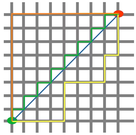
The blue line illustrates the Eucliden distance between the green and red dot. Otherwise you can also move over the orange, green or yellow line from the green point to the red point. The lines correspond to the manhatten distance. The length is equal.
Determining the Neighbors
To determine the similarity between two instances, we will use the Euclidean distance.
We can calculate the Euclidean distance with the function norm of the module np.linalg:
def distance(instance1, instance2):
    """ Calculates the Eucledian distance between two instances"""
    return np.linalg.norm(np.subtract(instance1, instance2))

print(distance([3, 5], [1, 1]))
print(distance(learn_data[3], learn_data[44]))
OUTPUT:
4.47213595499958
3.4190641994557516
The function get_neighbors returns a list with k neighbors, which are closest to the instance test_instance:
def get_neighbors(training_set,
                  labels,
                  test_instance,
                  k,
                  distance):
    """
    get_neighors calculates a list of the k nearest neighbors
    of an instance 'test_instance'.
    The function returns a list of k 3-tuples.
    Each 3-tuples consists of (index, dist, label)
    where
    index    is the index from the training_set,
    dist     is the distance between the test_instance and the
             instance training_set[index]
    distance is a reference to a function used to calculate the
             distances
    """
    distances = []
    for index in range(len(training_set)):
        dist = distance(test_instance, training_set[index])
        distances.append((training_set[index], dist, labels[index]))
    distances.sort(key=lambda x: x[1])
    neighbors = distances[:k]
    return neighbors
We will test the function with our iris samples:
for i in range(5):
    neighbors = get_neighbors(learn_data,
                              learn_labels,
                              test_data[i],
                              3,
                              distance=distance)
    print("Index:         ",i,'\n',
          "Testset Data:  ",test_data[i],'\n',
          "Testset Label: ",test_labels[i],'\n',
          "Neighbors:      ",neighbors,'\n')
OUTPUT:
Index:          0
 Testset Data:   [5.7 2.8 4.1 1.3]
 Testset Label:  1
 Neighbors:       [(array([5.7, 2.9, 4.2, 1.3]), 0.14142135623730995, 1), (array([5.6, 2.7, 4.2, 1.3]), 0.17320508075688815, 1), (array([5.6, 3. , 4.1, 1.3]), 0.22360679774997935, 1)]

Index:          1
 Testset Data:   [6.5 3.  5.5 1.8]
 Testset Label:  2
 Neighbors:       [(array([6.4, 3.1, 5.5, 1.8]), 0.1414213562373093, 2), (array([6.3, 2.9, 5.6, 1.8]), 0.24494897427831785, 2), (array([6.5, 3. , 5.2, 2. ]), 0.3605551275463988, 2)]

Index:          2
 Testset Data:   [6.3 2.3 4.4 1.3]
 Testset Label:  1
 Neighbors:       [(array([6.2, 2.2, 4.5, 1.5]), 0.2645751311064586, 1), (array([6.3, 2.5, 4.9, 1.5]), 0.574456264653803, 1), (array([6. , 2.2, 4. , 1. ]), 0.5916079783099617, 1)]

Index:          3
 Testset Data:   [6.4 2.9 4.3 1.3]
 Testset Label:  1
 Neighbors:       [(array([6.2, 2.9, 4.3, 1.3]), 0.20000000000000018, 1), (array([6.6, 3. , 4.4, 1.4]), 0.2645751311064587, 1), (array([6.6, 2.9, 4.6, 1.3]), 0.3605551275463984, 1)]

Index:          4
 Testset Data:   [5.6 2.8 4.9 2. ]
 Testset Label:  2
 Neighbors:       [(array([5.8, 2.7, 5.1, 1.9]), 0.31622776601683755, 2), (array([5.8, 2.7, 5.1, 1.9]), 0.31622776601683755, 2), (array([5.7, 2.5, 5. , 2. ]), 0.33166247903553986, 2)]
Voting to get a Single Result
We will write a vote function now. This functions uses the class Counter from collections to count the quantity of the classes inside of an instance list. This instance list will be the neighbors of course. The function vote returns the most common class:
from collections import Counter

def vote(neighbors):
    class_counter = Counter()
    for neighbor in neighbors:
        class_counter[neighbor[2]] += 1
    return class_counter.most_common(1)[0][0]
We will test 'vote' on our test data:
for i in range(n_test_samples):
    neighbors = get_neighbors(learn_data,
                              learn_labels,
                              test_data[i],
                              3,
                              distance=distance)
    print("index: ", i,
          ", result of vote: ", vote(neighbors),
          ", label: ", test_labels[i],
          ", data: ", test_data[i])
OUTPUT:
index:  0 , result of vote:  1 , label:  1 , data:  [5.7 2.8 4.1 1.3]
index:  1 , result of vote:  2 , label:  2 , data:  [6.5 3.  5.5 1.8]
index:  2 , result of vote:  1 , label:  1 , data:  [6.3 2.3 4.4 1.3]
index:  3 , result of vote:  1 , label:  1 , data:  [6.4 2.9 4.3 1.3]
index:  4 , result of vote:  2 , label:  2 , data:  [5.6 2.8 4.9 2. ]
index:  5 , result of vote:  2 , label:  2 , data:  [5.9 3.  5.1 1.8]
index:  6 , result of vote:  0 , label:  0 , data:  [5.4 3.4 1.7 0.2]
index:  7 , result of vote:  1 , label:  1 , data:  [6.1 2.8 4.  1.3]
index:  8 , result of vote:  1 , label:  2 , data:  [4.9 2.5 4.5 1.7]
index:  9 , result of vote:  0 , label:  0 , data:  [5.8 4.  1.2 0.2]
index:  10 , result of vote:  1 , label:  1 , data:  [5.8 2.6 4.  1.2]
index:  11 , result of vote:  2 , label:  2 , data:  [7.1 3.  5.9 2.1]
We can see that the predictions correspond to the labelled results, except in case of the item with the index 8.
'vote_prob' is a function like 'vote' but returns the class name and the probability for this class:
def vote_prob(neighbors):
    class_counter = Counter()
    for neighbor in neighbors:
        class_counter[neighbor[2]] += 1
    labels, votes = zip(*class_counter.most_common())
    winner = class_counter.most_common(1)[0][0]
    votes4winner = class_counter.most_common(1)[0][1]
    return winner, votes4winner/sum(votes)
for i in range(n_test_samples):
    neighbors = get_neighbors(learn_data,
                              learn_labels,
                              test_data[i],
                              5,
                              distance=distance)
    print("index: ", i,
          ", vote_prob: ", vote_prob(neighbors),
          ", label: ", test_labels[i],
          ", data: ", test_data[i])
OUTPUT:
index:  0 , vote_prob:  (1, 1.0) , label:  1 , data:  [5.7 2.8 4.1 1.3]
index:  1 , vote_prob:  (2, 1.0) , label:  2 , data:  [6.5 3.  5.5 1.8]
index:  2 , vote_prob:  (1, 1.0) , label:  1 , data:  [6.3 2.3 4.4 1.3]
index:  3 , vote_prob:  (1, 1.0) , label:  1 , data:  [6.4 2.9 4.3 1.3]
index:  4 , vote_prob:  (2, 1.0) , label:  2 , data:  [5.6 2.8 4.9 2. ]
index:  5 , vote_prob:  (2, 0.8) , label:  2 , data:  [5.9 3.  5.1 1.8]
index:  6 , vote_prob:  (0, 1.0) , label:  0 , data:  [5.4 3.4 1.7 0.2]
index:  7 , vote_prob:  (1, 1.0) , label:  1 , data:  [6.1 2.8 4.  1.3]
index:  8 , vote_prob:  (1, 1.0) , label:  2 , data:  [4.9 2.5 4.5 1.7]
index:  9 , vote_prob:  (0, 1.0) , label:  0 , data:  [5.8 4.  1.2 0.2]
index:  10 , vote_prob:  (1, 1.0) , label:  1 , data:  [5.8 2.6 4.  1.2]
index:  11 , vote_prob:  (2, 1.0) , label:  2 , data:  [7.1 3.  5.9 2.1]
The Weighted Nearest Neighbour Classifier
We looked only at k items in the vicinity of an unknown object „UO", and had a majority vote. Using the majority vote has shown quite efficient in our previous example, but this didn't take into account the following reasoning: The farther a neighbor is, the more it "deviates" from the "real" result. Or in other words, we can trust the closest neighbors more than the farther ones. Let's assume, we have 11 neighbors of an unknown item UO. The closest five neighbors belong to a class A and all the other six, which are farther away belong to a class B. What class should be assigned to UO? The previous approach says B, because we have a 6 to 5 vote in favor of B. On the other hand the closest 5 are all A and this should count more.
To pursue this strategy, we can assign weights to the neighbors in the following way: The nearest neighbor of an instance gets a weight $1 / 1$, the second closest gets a weight of $1 / 2$ and then going on up to $1/k$ for the farthest away neighbor.
This means that we are using the harmonic series as weights:
We implement this in the following function:
def vote_harmonic_weights(neighbors, all_results=True):
    class_counter = Counter()
    number_of_neighbors = len(neighbors)
    for index in range(number_of_neighbors):
        class_counter[neighbors[index][2]] += 1/(index+1)
    labels, votes = zip(*class_counter.most_common())
    #print(labels, votes)
    winner = class_counter.most_common(1)[0][0]
    votes4winner = class_counter.most_common(1)[0][1]
    if all_results:
        total = sum(class_counter.values(), 0.0)
        for key in class_counter:
             class_counter[key] /= total
        return winner, class_counter.most_common()
    else:
        return winner, votes4winner / sum(votes)
for i in range(n_test_samples):
    neighbors = get_neighbors(learn_data,
                              learn_labels,
                              test_data[i],
                              6,
                              distance=distance)
    print("index: ", i,
          ", result of vote: ",
          vote_harmonic_weights(neighbors,
                                all_results=True))
OUTPUT:
index:  0 , result of vote:  (1, [(1, 1.0)])
index:  1 , result of vote:  (2, [(2, 1.0)])
index:  2 , result of vote:  (1, [(1, 1.0)])
index:  3 , result of vote:  (1, [(1, 1.0)])
index:  4 , result of vote:  (2, [(2, 0.9319727891156463), (1, 0.06802721088435375)])
index:  5 , result of vote:  (2, [(2, 0.8503401360544217), (1, 0.14965986394557826)])
index:  6 , result of vote:  (0, [(0, 1.0)])
index:  7 , result of vote:  (1, [(1, 1.0)])
index:  8 , result of vote:  (1, [(1, 1.0)])
index:  9 , result of vote:  (0, [(0, 1.0)])
index:  10 , result of vote:  (1, [(1, 1.0)])
index:  11 , result of vote:  (2, [(2, 1.0)])
The previous approach took only the ranking of the neighbors according to their distance in account. We can improve the voting by using the actual distance. To this purpos we will write a new voting function:
def vote_distance_weights(neighbors, all_results=True):
    class_counter = Counter()
    number_of_neighbors = len(neighbors)
    for index in range(number_of_neighbors):
        dist = neighbors[index][1]
        label = neighbors[index][2]
        class_counter[label] += 1 / (dist**2 + 1)
    labels, votes = zip(*class_counter.most_common())
    #print(labels, votes)
    winner = class_counter.most_common(1)[0][0]
    votes4winner = class_counter.most_common(1)[0][1]
    if all_results:
        total = sum(class_counter.values(), 0.0)
        for key in class_counter:
             class_counter[key] /= total
        return winner, class_counter.most_common()
    else:
        return winner, votes4winner / sum(votes)
for i in range(n_test_samples):
    neighbors = get_neighbors(learn_data,
                              learn_labels,
                              test_data[i],
                              6,
                              distance=distance)
    print("index: ", i,
          ", result of vote: ",
          vote_distance_weights(neighbors,
                                all_results=True))
OUTPUT:
index:  0 , result of vote:  (1, [(1, 1.0)])
index:  1 , result of vote:  (2, [(2, 1.0)])
index:  2 , result of vote:  (1, [(1, 1.0)])
index:  3 , result of vote:  (1, [(1, 1.0)])
index:  4 , result of vote:  (2, [(2, 0.8490154592118361), (1, 0.15098454078816387)])
index:  5 , result of vote:  (2, [(2, 0.6736137462184479), (1, 0.3263862537815521)])
index:  6 , result of vote:  (0, [(0, 1.0)])
index:  7 , result of vote:  (1, [(1, 1.0)])
index:  8 , result of vote:  (1, [(1, 1.0)])
index:  9 , result of vote:  (0, [(0, 1.0)])
index:  10 , result of vote:  (1, [(1, 1.0)])
index:  11 , result of vote:  (2, [(2, 1.0)])
Live Python training

Enjoying this page? We offer live Python training courses covering the content of this site.
See our Python training courses
Exercise and Example: Classifying Fruits with K-Nearest Neighbors

Dataset: Generate a dataset containing information about fruits with three features: sweetness, acidity, and weight (in grams). We'll consider three types of fruits: "Apple", "Lemon", and "Mango".
Objective: Build a K-nearest neighbors classifier to predict the type of fruit based on its sweetness, acidity, and weight.
We will first create random data with fruits and corresponding data:
We use the Brix scale for the sweetness of apples.
import numpy as np

np.random.seed(42)

def create_features(number_samples, *min_max_features):
    """ Creates an array with number_samples rows and len(min_max_features) columns """
    features = []
    for min_val, max_val,rounding in min_max_features:
        features.append(np.random.uniform(min_val, max_val, number_samples).round(rounding))
    result = np.column_stack(features)
    return result

num_apples, num_mangos, num_lemons = 150, 150, 150
sweetness = (10, 18, 0)
acidity = 3.4, 4, 2
weight = 140.0, 250.0, 0
apples = create_features(num_apples, sweetness, acidity, weight)
apples[:20] # The first 20 fruits
OUTPUT:
array([[ 13.  ,   3.94, 146.  ],
       [ 18.  ,   3.54, 198.  ],
       [ 16.  ,   3.49, 199.  ],
       [ 15.  ,   3.69, 210.  ],
       [ 11.  ,   3.99, 220.  ],
       [ 11.  ,   3.55, 247.  ],
       [ 10.  ,   3.8 , 197.  ],
       [ 17.  ,   3.86, 176.  ],
       [ 15.  ,   3.54, 227.  ],
       [ 16.  ,   3.84, 170.  ],
       [ 10.  ,   3.62, 188.  ],
       [ 18.  ,   3.78, 149.  ],
       [ 17.  ,   3.78, 143.  ],
       [ 12.  ,   3.72, 246.  ],
       [ 11.  ,   3.45, 232.  ],
       [ 11.  ,   3.9 , 217.  ],
       [ 12.  ,   3.59, 185.  ],
       [ 14.  ,   3.51, 159.  ],
       [ 13.  ,   3.42, 157.  ],
       [ 12.  ,   3.75, 168.  ]])
sweetness = (6, 14, 0)
acidity = 3.6, 6, 1       # should be between 5.8 and 6
weight = 100.0, 300.0, 0
mangos = create_features(num_mangos, sweetness, acidity, weight)

sweetness = (6, 12, 0)
acidity = 2.0, 2.6, 1
weight = 130, 170, 0
lemons = create_features(num_lemons, sweetness, acidity, weight)
from sklearn.model_selection import train_test_split
from sklearn.preprocessing import StandardScaler

# Combine the data and create labels
X = np.vstack((apples, mangos, lemons))
y = np.array(['Apple'] * num_apples + ['Mango'] * num_mangos + ['Lemon'] * num_lemons)

# Split the data into training and testing sets
X_train, X_test, y_train, y_test = train_test_split(X, y, test_size=0.2, random_state=42)
Before we go on with classifying our data, we will write the data to a csv file for future usage:
import pandas as pd

# Define the DataFrame
df = pd.DataFrame(X, columns=['Sweetness', 'Acidity', 'Weight'])
df['Fruit'] = y

# Write DataFrame to CSV file
df.to_csv('data/fruits_data.csv', index=False)
We will classify our data now with our get_neighbors function:
n_test_samples = len(X_test)

for i in range(20):
    neighbors = get_neighbors(X_train,
                              y_train,
                              X_test[i],
                              6,
                              distance=distance)

    print("index: ", i,
          ", result of vote: ",
          vote_harmonic_weights(neighbors,
                                all_results=True))
OUTPUT:
index:  0 , result of vote:  ('Lemon', [('Lemon', 1.0)])
index:  1 , result of vote:  ('Lemon', [('Lemon', 1.0)])
index:  2 , result of vote:  ('Apple', [('Apple', 0.5442176870748299), ('Mango', 0.4557823129251701)])
index:  3 , result of vote:  ('Apple', [('Apple', 0.9319727891156463), ('Mango', 0.06802721088435375)])
index:  4 , result of vote:  ('Lemon', [('Lemon', 1.0)])
index:  5 , result of vote:  ('Mango', [('Mango', 0.6802721088435374), ('Lemon', 0.18367346938775508), ('Apple', 0.13605442176870747)])
index:  6 , result of vote:  ('Lemon', [('Lemon', 1.0)])
index:  7 , result of vote:  ('Lemon', [('Lemon', 1.0)])
index:  8 , result of vote:  ('Apple', [('Apple', 0.693877551020408), ('Mango', 0.3061224489795918)])
index:  9 , result of vote:  ('Mango', [('Mango', 1.0)])
index:  10 , result of vote:  ('Apple', [('Apple', 0.7619047619047619), ('Mango', 0.23809523809523805)])
index:  11 , result of vote:  ('Lemon', [('Lemon', 1.0)])
index:  12 , result of vote:  ('Apple', [('Apple', 1.0)])
index:  13 , result of vote:  ('Apple', [('Apple', 1.0)])
index:  14 , result of vote:  ('Lemon', [('Lemon', 1.0)])
index:  15 , result of vote:  ('Lemon', [('Lemon', 0.6802721088435374), ('Mango', 0.18367346938775508), ('Apple', 0.13605442176870747)])
index:  16 , result of vote:  ('Mango', [('Mango', 0.5578231292517006), ('Apple', 0.44217687074829926)])
index:  17 , result of vote:  ('Apple', [('Apple', 0.9319727891156463), ('Mango', 0.06802721088435375)])
index:  18 , result of vote:  ('Apple', [('Apple', 0.9319727891156463), ('Mango', 0.06802721088435375)])
index:  19 , result of vote:  ('Apple', [('Apple', 0.9319727891156463), ('Lemon', 0.06802721088435375)])
To evaluate our classifificatione we write an evaluate function now:
def evaluate(X_train, X_test, y_train, y_test, threshold=0):
    """
    Evaluate the performance of a K-nearest neighbors classifier.

    Parameters:
        X_train (ndarray): Training features.
        X_test (ndarray): Testing features.
        y_train (ndarray): Training labels.
        y_test (ndarray): Testing labels.
        threshold (float): Threshold for decision-making confidence (default: 0).
                           If the probability of the predicted class is below this threshold,
                           the sample will be marked as undecided.

    Returns:
        dict: A dictionary containing counts of correct predictions, wrong predictions,
              and undecided predictions.

    Note:
        The function assumes that there is another function called get_neighbors that
        retrieves the k-nearest neighbors for each sample, and the distance metric used
        by the K-nearest neighbors algorithm is defined in a variable called 'distance'.
    """
    evaluation = dict(corrects=0, wrongs=0, undecided=0)
    n_test_samples = len(X_test)
    for i in range(n_test_samples):
        neighbors = get_neighbors(X_train,
                                  y_train,
                                  X_test[i],
                                  6,
                                  distance=distance)
        class_label, probability = vote_distance_weights(neighbors, all_results=False)
        if class_label == y_test[i]:
            if probability >= threshold:
                evaluation['corrects'] += 1
            else:
                evaluation['undecided'] += 1
        else:
            if probability >= threshold:
                evaluation['wrongs'] += 1
            else:
                evaluation['undecided'] += 1
    return evaluation


evaluate(X_train, X_test, y_train, y_test, 0.5)
OUTPUT:
{'corrects': 71, 'wrongs': 17, 'undecided': 2}
evaluate(X_train, X_test, y_train, y_test, 0.9)
OUTPUT:
{'corrects': 49, 'wrongs': 3, 'undecided': 38}
kNN in Linguistics
The next example comes from computer linguistics. We show how we can use a k-nearest neighbor classifier to recognize misspelled words.
We use a module called levenshtein, which we have implemented in our tutorial on Levenshtein Distance.
from levenshtein import levenshtein

cities = open("data/city_names.txt").readlines()
cities = [city.strip() for city in cities]

for city in ["Freiburg", "Frieburg", "Freiborg",
             "Hamborg", "Sahrluis"]:
    neighbors = get_neighbors(cities,
                              cities,
                              city,
                              2,
                              distance=levenshtein)

    print("vote_distance_weights: ", vote_distance_weights(neighbors))
OUTPUT:
vote_distance_weights:  ('Freiburg', [('Freiburg', 0.6666666666666666), ('Freiberg', 0.3333333333333333)])
vote_distance_weights:  ('Freiburg', [('Freiburg', 0.6666666666666666), ('Lüneburg', 0.3333333333333333)])
vote_distance_weights:  ('Freiburg', [('Freiburg', 0.5), ('Freiberg', 0.5)])
vote_distance_weights:  ('Hamburg', [('Hamburg', 0.7142857142857143), ('Bamberg', 0.28571428571428575)])
vote_distance_weights:  ('Saarlouis', [('Saarlouis', 0.8387096774193549), ('Bayreuth', 0.16129032258064516)])
You may wonder why the city of Freiburg has not been recognized. The reaons is that our data file with the city names contains only "Freiburg im Breisgau". If you add "Freiburg" as an entry, it will be recognized as well.
Marvin and James introduce us to our next example:

Can you help Marvin and James?

You will need an English dictionary and a k-nearest Neighbor classifier to solve this problem. If you work under Linux (especially Ubuntu), you can find a file with a British-English dictionary under /usr/share/dict/british-english. Windows users and others can download the file as
/data1/british-english.txtWe use extremely misspelled words in the following example. We see that our simple vote_prob function is doing well only in two cases: In correcting "holpposs" to "helpless" and "blagrufoo" to "barefoot". Whereas our distance voting is doing well in all cases. Okay, we have to admit that we had "liberty" in mind, when we wrote "liberdi", but suggesting "liberal" is a good choice.
words = []
with open("british-english.txt") as fh:
    for line in fh:
        word = line.strip()
        words.append(word)

for word in ["holpful", "kundnoss", "holpposs", "thoes", "innerstand",
             "blagrufoo", "liberdi"]:
    neighbors = get_neighbors(words,
                              words,
                              word,
                              3,
                              distance=levenshtein)

    print("vote_distance_weights: ", vote_distance_weights(neighbors,
                                                           all_results=False))
    print("vote_prob: ", vote_prob(neighbors))
    print("vote_distance_weights: ", vote_distance_weights(neighbors))
OUTPUT:
vote_distance_weights:  ('helpful', 0.5555555555555556)
vote_prob:  ('helpful', 0.3333333333333333)
vote_distance_weights:  ('helpful', [('helpful', 0.5555555555555556), ('doleful', 0.22222222222222227), ('hopeful', 0.22222222222222227)])
vote_distance_weights:  ('kindness', 0.5)
vote_prob:  ('kindness', 0.3333333333333333)
vote_distance_weights:  ('kindness', [('kindness', 0.5), ('fondness', 0.25), ('kudos', 0.25)])
vote_distance_weights:  ('helpless', 0.3333333333333333)
vote_prob:  ('helpless', 0.3333333333333333)
vote_distance_weights:  ('helpless', [('helpless', 0.3333333333333333), ("hippo's", 0.3333333333333333), ('hippos', 0.3333333333333333)])
vote_distance_weights:  ('hoes', 0.3333333333333333)
vote_prob:  ('hoes', 0.3333333333333333)
vote_distance_weights:  ('hoes', [('hoes', 0.3333333333333333), ('shoes', 0.3333333333333333), ('thees', 0.3333333333333333)])
vote_distance_weights:  ('understand', 0.5)
vote_prob:  ('understand', 0.3333333333333333)
vote_distance_weights:  ('understand', [('understand', 0.5), ('interstate', 0.25), ('understands', 0.25)])
vote_distance_weights:  ('barefoot', 0.4333333333333333)
vote_prob:  ('barefoot', 0.3333333333333333)
vote_distance_weights:  ('barefoot', [('barefoot', 0.4333333333333333), ('Baguio', 0.2833333333333333), ('Blackfoot', 0.2833333333333333)])
vote_distance_weights:  ('liberal', 0.4)
vote_prob:  ('liberal', 0.3333333333333333)
vote_distance_weights:  ('liberal', [('liberal', 0.4), ('liberty', 0.4), ('Hibernia', 0.2)])
Live Python training
Enjoying this page? We offer live Python training courses covering the content of this site.
Upcoming online Courses
See our Python training courses