37. Expectation Maximization and Gaussian Mixture Models (GMM)

By Tobias Schlagenhauf. Last modified: 22 Feb 2022.

Context and Key Concepts

The Gaussian Mixture Models (GMM) algorithm is an unsupervised learning algorithm since we do not know any values of a target feature. Further, the GMM is categorized into the clustering algorithms, since it can be used to find clusters in the data. Key concepts you should have heard about are:

• Multivariate Gaussian Distribution
• Covariance Matrix
• Mean vector of multivariate data

Live Python training

Enjoying this page? We offer live Python training courses covering the content of this site.

See: Live Python courses overview

Enrol here

What are Gaussian Mixture models

We want to use Gaussian Mixture models to find clusters in a dataset from which we know (or assume to know) the number of clusters enclosed in this dataset, but we do not know where these clusters are as well as how they are shaped. Finding these clusters is the task of GMM and since we don't have any information instead of the number of clusters, the GMM is an unsupervised approach. To accomplish that, we try to fit a mixture of gaussians to our dataset. That is, we try to find a number of gaussian distributions which can be used to describe the shape of our dataset. A critical point for the understanding is that these gaussian shaped clusters must not be circular shaped as for instance in the KNN approach but can have all shapes a multivariate Gaussian distribution can take. That is, a circle can only change in its diameter whilst a GMM model can (because of its covariance matrix) model all ellipsoid shapes as well. See the following illustration for an example in the two dimensional space.

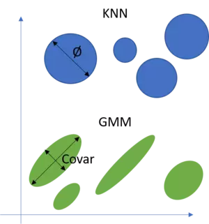
What I have omitted in this illustration is that the position in space of KNN and GMM models is defined by their mean vector. Hence the mean vector gives the space whilst the diameter respectively the covariance matrix defines the shape of KNN and GMM models.

So if we consider an arbitrary dataset like the following:

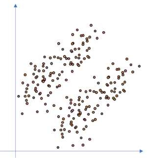
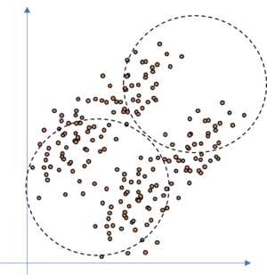
How precise can we fit a KNN model to this kind of dataset, if we assume that there are two clusters in the dataset? Well, not so precise since we have overlapping areas where the KNN model is not accurate. This is due to the fact that the KNN clusters are circular shaped whilst the data is of ellipsoid shape. It may even happen that the KNN totally fails as illustrated in the following figure.

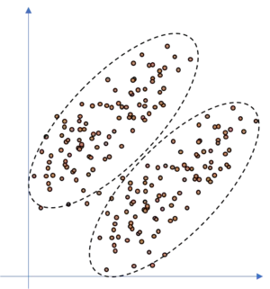
If we would fit ellipsoids to the data, as we do with the GMM approach, we would be able to model the dataset well, as illustrated in the following figure.

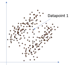
Another weak point of KNN in its original form is that each point is allocated to one cluster, that is, each point either belongs to cluster one or two in our example. So assume, we add some more datapoints in between the two clusters in our illustration above. As you can see, we can still assume that there are two clusters, but in the space between the two clusters are some points where it is not totally clear to which cluster they belong. Tackling this dataset with an classical KNN approach would lead to the result, that each datapoint is allocated to cluster one or cluster two respectively and therewith the KNN algorithm would find a hard cut-off border between the two clusters. Though, as you can see, this is probably not correct for all datapoints since we rather would say that for instance datapoint 1 has a probability of 60% to belong to cluster one and a probability of 40% to belong to cluster two. Hence we want to assign probabilities to the datapoints.

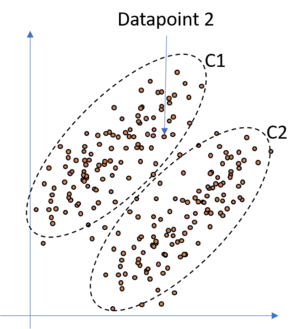
In such a case, a classical KNN approach is rather useless and we need something let's say more flexible or smth. which adds more likelihood to our clustering. Fortunately,the GMM is such a model. Since we do not simply try to model the data with circles but add gaussians to our data this allows us to allocate to each point a likelihood to belong to each of the gaussians. It is clear, and we know, that the closer a datapoint is to one gaussian, the higher is the probability that this point actually belongs to this gaussian and the less is the probability that this point belongs to the other gaussian. Therefore, consider the following illustration where we have added a GMM to the above data and highlighted point 2. This point is much more likely to belong to cluster/gaussian one (C1) than to cluster/gaussian two (C2). Hence, if we would calculate the probability for this point for each cluster we would get smth. like: With a probability of 99% This point belongs to cluster one, and with a probability of 1% to cluster two.

So let's quickly summarize and recapitulate in which cases we want to use a GMM over a classical KNN approach. If we have data where we assume that the clusters are not defined by simple circles but by more complex, ellipsoid shapes, we prefer the GMM approach over the KNN approach. Additionally, if we want to have soft cut-off borders and therewith probabilities, that is, if we want to know the probability of a datapoint to belong to each of our clusters, we prefer the GMM over the KNN approach. Hence, if there arise the two buzz words probabilities and non-circular during our model selection discussion, we should strongly check the use of the GMM.

So now that we know that we should check the usage of the GMM approach if we want to allocate probabilities to our clusterings or if there are non-circular clusters, we should take a look at how we can build a GMM model. This is derived in the next section of this tutorial. So much for that: We follow a approach called Expectation Maximization (EM).

Maths behind Gaussian Mixture Models (GMM)

To understand the maths behind the GMM concept I strongly recommend to watch the video of Prof. Alexander Ihler about Gaussian Mixture Models and EM. This video gives a perfect insight into what is going on during the calculations of a GMM and I want to build the following steps on top of that video. After you have red the above section and watched this video you will understand the following pseudocode.

So we know that we have to run the E-Step and the M-Step iteratively and maximize the log likelihood function until it converges. Though, we will go into more detail about what is going on during these two steps and how we can compute this in python for one and more dimensional datasets.

I will quickly show the E, M steps here.

1. Decide how many sources/clusters (c) you want to fit to your data
2. Initialize the parameters mean $\mu_c$, covariance $\Sigma_c$, and fraction_per_class $\pi_c$ per cluster c

$\underline{E-Step}$

1. Calculate for each datapoint $x_i$ the probability $r_{ic}$ that datapoint $x_i$ belongs to cluster c with:

   $$r_{ic} = \frac{\pi_c N(\boldsymbol{x_i} \ | \ \boldsymbol{\mu_c},\boldsymbol{\Sigma_c})}{\Sigma_{k=1}^K \pi_k N(\boldsymbol{x_i \ | \ \boldsymbol{\mu_k},\boldsymbol{\Sigma_k}})}$$ where $N(\boldsymbol{x} \ | \ \boldsymbol{\mu},\boldsymbol{\Sigma})$ describes the mulitvariate Gaussian with:

   $$N(\boldsymbol{x_i},\boldsymbol{\mu_c},\boldsymbol{\Sigma_c}) \ = \ \frac{1}{(2\pi)^{\frac{n}{2}}|\Sigma_c|^{\frac{1}{2}}}exp(-\frac{1}{2}(\boldsymbol{x_i}-\boldsymbol{\mu_c})^T\boldsymbol{\Sigma_c^{-1}}(\boldsymbol{x_i}-\boldsymbol{\mu_c}))$$

   $r_{ic}$ gives us for each datapoint $x_i$ the measure of: $\frac{Probability \ that \ x_i \ belongs \ to \ class \ c}{Probability \ of \ x_i \ over \ all \ classes}$ hence if $x_i$ is very close to one gaussian c, it will get a high $r_{ic}$ value for this gaussian and relatively low values otherwise.

   $\underline{M-Step}$

   For each cluster c: Calculate the total weight $m_c$ (loosely speaking the fraction of points allocated to cluster c) and update $\pi_c$, $\mu_c$, and $\Sigma_c$ using $r_{ic}$ with:

   $$m_c \ = \ \Sigma_i r_{ic}$$

   $$\pi_c \ = \ \frac{m_c}{m}$$

   $$\boldsymbol{\mu_c} \ = \ \frac{1}{m_c}\Sigma_i r_{ic} \boldsymbol{x_i} $$

   $$\boldsymbol{\Sigma_c} \ = \ \frac{1}{m_c}\Sigma_i r_{ic}(\boldsymbol{x_i}-\boldsymbol{\mu_c})^T(\boldsymbol{x_i}-\boldsymbol{\mu_c})$$

   Mind that you have to use the updated means in this last formula.

   Iteratively repeat the E and M step until the log-likelihood function of our model converges where the log likelihood is computed with:

   $$ln \ p(\boldsymbol{X} \ | \ \boldsymbol{\pi},\boldsymbol{\mu},\boldsymbol{\Sigma}) \ = \ \Sigma_{i=1}^N \ ln(\Sigma_{k=1}^K \pi_k N(\boldsymbol{x_i} \ | \ \boldsymbol{\mu_k},\boldsymbol{\Sigma_k}))$$

Live Python training

Enjoying this page? We offer live Python training courses covering the content of this site.

See: Live Python courses overview

Upcoming online Courses

Python Text Processing Course

Enrol here

GMM in Python from scratch

To understand how we can implement the above in Python, we best go through the single steps, step by step. Therefore, we best start with the following situation:

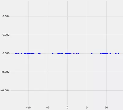
What can you say about this data? Well, we may see that there are kind of three data clusters. Further, we know that our goal is to automatically fit gaussians (in this case it should be three) to this dataset. Now first of all, lets draw three randomly drawn gaussians on top of that data and see if this brings us any further.

What do we have now? Well, we have the datapoints and we have three randomly chosen gaussian models on top of that datapoints. Remember that we want to have three gaussian models fitted to our three data-clusters. So how can we cause these three randomly chosen guassians to fit the data automatically? Well, here we use an approach called Expectation-Maximization (EM). This approach can, in principal, be used for many different models but it turns out that it is especially popular for the fitting of a bunch of Gaussians to data. I won't go into detail about the principal EM algorithm itself and will only talk about its application for GMM. If you want to read more about it I recommend the chapter about General Statement of EM Algorithm in Mitchel (1997) pp.194. But don't panic, in principal it works always the same.

Ok, now we know that we want to use something called Expectation Maximization. This term consists of two parts: Expectation and Maximzation. Well, how can we combine the data and above randomly drawn gaussians with the first term Expectation? Lets try to simply calculate the probability for each datapoint in our dataset for each gaussian, that it the probability that this datapoint belongs to each of the three gaussians. Since we have to store these probabilities somewhere, we introduce a new variable and call this variable $r$. We use $r$ for convenience purposes to kind of have a container where we can store the probability that datapoint $x_i$ belongs to gaussian $c$. We denote this probability with $r_{ic}$. What we get as result is an nxK array where n denotes the number of datapoints in $x$ and K denotes the number of clusters/gaussians. Hm let's try this for our data and see what we get.

import numpy as np
from scipy.stats import norm
np.random.seed(0)

X = np.linspace(-5,5,num=20)
X0 = X*np.random.rand(len(X))+10 # Create data cluster 1
X1 = X*np.random.rand(len(X))-10 # Create data cluster 2
X2 = X*np.random.rand(len(X)) # Create data cluster 3
X_tot = np.stack((X0,X1,X2)).flatten() # Combine the clusters to get the random datapoints from above



"""Create the array r with dimensionality nxK"""
r = np.zeros((len(X_tot),3))  
print('Dimensionality','=',np.shape(r))

"""Instantiate the random gaussians"""

gauss_1 = norm(loc=-5,scale=5) 
gauss_2 = norm(loc=8,scale=3)
gauss_3 = norm(loc=1.5,scale=1)

"""
Probability for each datapoint x_i to belong to gaussian g 
"""
for c,g in zip(range(3),[gauss_1,gauss_2,gauss_3]):
    r[:,c] = g.pdf(X_tot) # Write the probability that x belongs to gaussian c in column c. 
                          # Therewith we get a 60x3 array filled with the probability that each x_i belongs to one of the gaussians
"""
Normalize the probabilities such that each row of r sums to 1
"""
for i in range(len(r)):
    r[i] = r[i]/np.sum(r,axis=1)[i] 

"""In the last calculation we normalized the probabilites r_ic. So each row i in r gives us the probability for x_i 
to belong to one gaussian (one column per gaussian). Since we want to know the probability that x_i belongs 
to gaussian g, we have to do smth. like a simple calculation of percentage where we want to know how likely it is in % that
x_i belongs to gaussian g. To realize this, we must dive the probability of each r_ic by the total probability r_i (this is done by 
summing up each row in r and divide each value r_ic by sum(np.sum(r,axis=1)[r_i] )). To get this,
look at the above plot and pick an arbitrary datapoint. Pick one gaussian and imagine the probability that this datapoint
belongs to this gaussian. This value will normally be small since the point is relatively far away right? So what is
the percentage that this point belongs to the chosen gaussian? --> Correct, the probability that this datapoint belongs to this 
gaussian divided by the sum of the probabilites for this datapoint for all three gaussians."""
    
print(r)
print(np.sum(r,axis=1)) # As we can see, as result each row sums up to one, just as we want it.

Dimensionality = (60, 3)
[[2.97644006e-02 9.70235407e-01 1.91912550e-07]
 [3.85713024e-02 9.61426220e-01 2.47747304e-06]
 [2.44002651e-02 9.75599713e-01 2.16252823e-08]
 [1.86909096e-02 9.81309090e-01 8.07574590e-10]
 [1.37640773e-02 9.86235923e-01 9.93606589e-12]
 [1.58674083e-02 9.84132592e-01 8.42447356e-11]
 [1.14191259e-02 9.88580874e-01 4.48947365e-13]
 [1.34349421e-02 9.86565058e-01 6.78305927e-12]
 [1.11995848e-02 9.88800415e-01 3.18533028e-13]
 [8.57645259e-03 9.91423547e-01 1.74498648e-15]
 [7.64696969e-03 9.92353030e-01 1.33051021e-16]
 [7.10275112e-03 9.92897249e-01 2.22285146e-17]
 [6.36154765e-03 9.93638452e-01 1.22221112e-18]
 [4.82376290e-03 9.95176237e-01 1.55549544e-22]
 [7.75866904e-03 9.92241331e-01 1.86665135e-16]
 [7.52759691e-03 9.92472403e-01 9.17205413e-17]
 [8.04550643e-03 9.91954494e-01 4.28205323e-16]
 [3.51864573e-03 9.96481354e-01 9.60903037e-30]
 [3.42631418e-03 9.96573686e-01 1.06921949e-30]
 [3.14390460e-03 9.96856095e-01 3.91217273e-35]
 [1.00000000e+00 2.67245688e-12 1.56443629e-57]
 [1.00000000e+00 4.26082753e-11 9.73970426e-49]
 [9.99999999e-01 1.40098281e-09 3.68939866e-38]
 [1.00000000e+00 2.65579518e-10 4.05324196e-43]
 [9.99999977e-01 2.25030673e-08 3.11711096e-30]
 [9.99999997e-01 2.52018974e-09 1.91287930e-36]
 [9.99999974e-01 2.59528826e-08 7.72534540e-30]
 [9.99999996e-01 4.22823192e-09 5.97494463e-35]
 [9.99999980e-01 1.98158593e-08 1.38414545e-30]
 [9.99999966e-01 3.43722391e-08 4.57504394e-29]
 [9.99999953e-01 4.74290492e-08 3.45975850e-28]
 [9.99999876e-01 1.24093364e-07 1.31878573e-25]
 [9.99999878e-01 1.21709730e-07 1.17161878e-25]
 [9.99999735e-01 2.65048706e-07 1.28402556e-23]
 [9.99999955e-01 4.53370639e-08 2.60841891e-28]
 [9.99999067e-01 9.33220139e-07 2.02379180e-20]
 [9.99998448e-01 1.55216175e-06 3.63693167e-19]
 [9.99997285e-01 2.71542629e-06 8.18923788e-18]
 [9.99955648e-01 4.43516655e-05 1.59283752e-11]
 [9.99987200e-01 1.28004505e-05 3.20565446e-14]
 [9.64689131e-01 9.53405294e-03 2.57768163e-02]
 [9.77001731e-01 7.96383733e-03 1.50344317e-02]
 [9.96373670e-01 2.97775078e-03 6.48579562e-04]
 [3.43634425e-01 2.15201653e-02 6.34845409e-01]
 [9.75390877e-01 8.19866977e-03 1.64104537e-02]
 [9.37822997e-01 1.19363656e-02 5.02406373e-02]
 [4.27396946e-01 2.18816340e-02 5.50721420e-01]
 [3.28570544e-01 2.14190231e-02 6.50010433e-01]
 [3.62198108e-01 2.16303800e-02 6.16171512e-01]
 [2.99837196e-01 2.11991858e-02 6.78963618e-01]
 [2.21768797e-01 2.04809383e-02 7.57750265e-01]
 [1.76497129e-01 2.01127714e-02 8.03390100e-01]
 [8.23252013e-02 2.50758227e-02 8.92598976e-01]
 [2.11943183e-01 2.03894641e-02 7.67667353e-01]
 [1.50351209e-01 2.00499057e-02 8.29598885e-01]
 [1.54779991e-01 2.00449518e-02 8.25175057e-01]
 [7.92109803e-02 5.93118654e-02 8.61477154e-01]
 [9.71905134e-02 2.18698473e-02 8.80939639e-01]
 [7.60625670e-02 4.95831879e-02 8.74354245e-01]
 [8.53513721e-02 2.40396004e-02 8.90609028e-01]]
[1. 1. 1. 1. 1. 1. 1. 1. 1. 1. 1. 1. 1. 1. 1. 1. 1. 1. 1. 1. 1. 1. 1. 1.
 1. 1. 1. 1. 1. 1. 1. 1. 1. 1. 1. 1. 1. 1. 1. 1. 1. 1. 1. 1. 1. 1. 1. 1.
 1. 1. 1. 1. 1. 1. 1. 1. 1. 1. 1. 1.]

So you see that we got an array $r$ where each row contains the probability that $x_i$ belongs to any of the gaussians $g$. Hence for each $x_i$ we get three probabilities, one for each gaussian $g$. Ok, so good for now. We now have three probabilities for each $x_i$ and that's fine. Recapitulate our initial goal: We want to fit as many gaussians to the data as we expect clusters in the dataset. Now, probably it would be the case that one cluster consists of more datapoints as another one and therewith the probability for each $x_i$ to belong to this "large" cluster is much greater than belonging to one of the others. How can we address this issue in our above code? Well, we simply code-in this probability by multiplying the probability for each $r_ic$ with the fraction of points we assume to belong to this cluster c. We denote this variable with $\pi_c$.

For illustration purposes, look at the following figure:

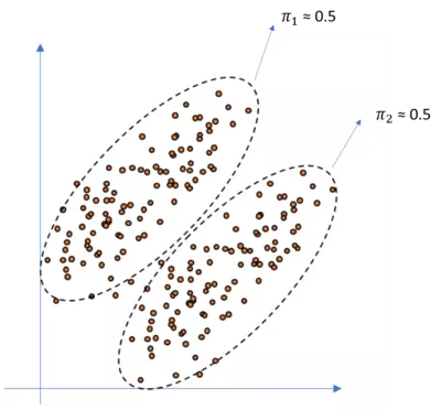
So as you can see, the points are approximately equally distributed over the two clusters and hence each $\mu_c$ is $\approx$ $0.5$. If the fractions where more unequally distributed like for instance if only two datapoints would belong to cluster 1, we would have more unbalanced $\mu$'s. The fractions must some to one. So let's implement these weighted classes in our code above. Since we do not know the actual values for our $mu$'s we have to set arbitrary values as well. We will set both $\mu_c$ to 0.5 here and hence we don't get any other results as above since the points are assumed to be equally distributed over the two clusters c.

import matplotlib.pyplot as plt
from matplotlib import style
style.use('fivethirtyeight')
import numpy as np
from scipy.stats import norm
np.random.seed(0)

X = np.linspace(-5,5,num=20)
X0 = X*np.random.rand(len(X))+10 # Create data cluster 1
X1 = X*np.random.rand(len(X))-10 # Create data cluster 2
X2 = X*np.random.rand(len(X)) # Create data cluster 3
X_tot = np.stack((X0,X1,X2)).flatten() # Combine the clusters to get the random datapoints from above



"""Create the array r with dimensionality nxK"""
r = np.zeros((len(X_tot),3))  
print('Dimensionality','=',np.shape(r))

"""Instantiate the random gaussians"""

gauss_1 = norm(loc=-5,scale=5) 
gauss_2 = norm(loc=8,scale=3)
gauss_3 = norm(loc=1.5,scale=1)

"""Instantiate the random pi_c"""
pi = np.array([1/3,1/3,1/3]) # We expect to have three clusters 


"""
Probability for each datapoint x_i to belong to gaussian g 
"""
for c,g,p in zip(range(3),[gauss_1,gauss_2,gauss_3],pi):
    r[:,c] = p*g.pdf(X_tot) # Write the probability that x belongs to gaussian c in column c. 
                          # Therewith we get a 60x3 array filled with the probability that each x_i belongs to one of the gaussians
"""
Normalize the probabilities such that each row of r sums to 1 and weight it by pi_c == the fraction of points belonging to 
cluster c
"""
for i in range(len(r)):
    r[i] = r[i]/(np.sum(pi)*np.sum(r,axis=1)[i])

"""In the last calculation we normalized the probabilites r_ic. So each row i in r gives us the probability for x_i 
to belong to one gaussian (one column per gaussian). Since we want to know the probability that x_i belongs 
to gaussian g, we have to do smth. like a simple calculation of percentage where we want to know how likely it is in % that
x_i belongs to gaussian g. To realize this we must dive the probability of each r_ic by the total probability r_i (this is done by 
summing up each row in r and divide each value r_ic by sum(np.sum(r,axis=1)[r_i] )). To get this,
look at the above plot and pick an arbitrary datapoint. Pick one gaussian and imagine the probability that this datapoint
belongs to this gaussian. This value will normally be small since the point is relatively far away right? So what is
the percentage that this point belongs to the chosen gaussian? --> Correct, the probability that this datapoint belongs to this 
gaussian divided by the sum of the probabilites for this datapoint and all three gaussians. Since we don't know how many
point belong to each cluster c and threwith to each gaussian c, we have to make assumptions and in this case simply said that we 
assume that the points are equally distributed over the three clusters."""
    
print(r)
print(np.sum(r,axis=1)) # As we can see, as result each row sums up to one, just as we want it.

Dimensionality = (60, 3)
[[2.97644006e-02 9.70235407e-01 1.91912550e-07]
 [3.85713024e-02 9.61426220e-01 2.47747304e-06]
 [2.44002651e-02 9.75599713e-01 2.16252823e-08]
 [1.86909096e-02 9.81309090e-01 8.07574590e-10]
 [1.37640773e-02 9.86235923e-01 9.93606589e-12]
 [1.58674083e-02 9.84132592e-01 8.42447356e-11]
 [1.14191259e-02 9.88580874e-01 4.48947365e-13]
 [1.34349421e-02 9.86565058e-01 6.78305927e-12]
 [1.11995848e-02 9.88800415e-01 3.18533028e-13]
 [8.57645259e-03 9.91423547e-01 1.74498648e-15]
 [7.64696969e-03 9.92353030e-01 1.33051021e-16]
 [7.10275112e-03 9.92897249e-01 2.22285146e-17]
 [6.36154765e-03 9.93638452e-01 1.22221112e-18]
 [4.82376290e-03 9.95176237e-01 1.55549544e-22]
 [7.75866904e-03 9.92241331e-01 1.86665135e-16]
 [7.52759691e-03 9.92472403e-01 9.17205413e-17]
 [8.04550643e-03 9.91954494e-01 4.28205323e-16]
 [3.51864573e-03 9.96481354e-01 9.60903037e-30]
 [3.42631418e-03 9.96573686e-01 1.06921949e-30]
 [3.14390460e-03 9.96856095e-01 3.91217273e-35]
 [1.00000000e+00 2.67245688e-12 1.56443629e-57]
 [1.00000000e+00 4.26082753e-11 9.73970426e-49]
 [9.99999999e-01 1.40098281e-09 3.68939866e-38]
 [1.00000000e+00 2.65579518e-10 4.05324196e-43]
 [9.99999977e-01 2.25030673e-08 3.11711096e-30]
 [9.99999997e-01 2.52018974e-09 1.91287930e-36]
 [9.99999974e-01 2.59528826e-08 7.72534540e-30]
 [9.99999996e-01 4.22823192e-09 5.97494463e-35]
 [9.99999980e-01 1.98158593e-08 1.38414545e-30]
 [9.99999966e-01 3.43722391e-08 4.57504394e-29]
 [9.99999953e-01 4.74290492e-08 3.45975850e-28]
 [9.99999876e-01 1.24093364e-07 1.31878573e-25]
 [9.99999878e-01 1.21709730e-07 1.17161878e-25]
 [9.99999735e-01 2.65048706e-07 1.28402556e-23]
 [9.99999955e-01 4.53370639e-08 2.60841891e-28]
 [9.99999067e-01 9.33220139e-07 2.02379180e-20]
 [9.99998448e-01 1.55216175e-06 3.63693167e-19]
 [9.99997285e-01 2.71542629e-06 8.18923788e-18]
 [9.99955648e-01 4.43516655e-05 1.59283752e-11]
 [9.99987200e-01 1.28004505e-05 3.20565446e-14]
 [9.64689131e-01 9.53405294e-03 2.57768163e-02]
 [9.77001731e-01 7.96383733e-03 1.50344317e-02]
 [9.96373670e-01 2.97775078e-03 6.48579562e-04]
 [3.43634425e-01 2.15201653e-02 6.34845409e-01]
 [9.75390877e-01 8.19866977e-03 1.64104537e-02]
 [9.37822997e-01 1.19363656e-02 5.02406373e-02]
 [4.27396946e-01 2.18816340e-02 5.50721420e-01]
 [3.28570544e-01 2.14190231e-02 6.50010433e-01]
 [3.62198108e-01 2.16303800e-02 6.16171512e-01]
 [2.99837196e-01 2.11991858e-02 6.78963618e-01]
 [2.21768797e-01 2.04809383e-02 7.57750265e-01]
 [1.76497129e-01 2.01127714e-02 8.03390100e-01]
 [8.23252013e-02 2.50758227e-02 8.92598976e-01]
 [2.11943183e-01 2.03894641e-02 7.67667353e-01]
 [1.50351209e-01 2.00499057e-02 8.29598885e-01]
 [1.54779991e-01 2.00449518e-02 8.25175057e-01]
 [7.92109803e-02 5.93118654e-02 8.61477154e-01]
 [9.71905134e-02 2.18698473e-02 8.80939639e-01]
 [7.60625670e-02 4.95831879e-02 8.74354245e-01]
 [8.53513721e-02 2.40396004e-02 8.90609028e-01]]
[1. 1. 1. 1. 1. 1. 1. 1. 1. 1. 1. 1. 1. 1. 1. 1. 1. 1. 1. 1. 1. 1. 1. 1.
 1. 1. 1. 1. 1. 1. 1. 1. 1. 1. 1. 1. 1. 1. 1. 1. 1. 1. 1. 1. 1. 1. 1. 1.
 1. 1. 1. 1. 1. 1. 1. 1. 1. 1. 1. 1.]

So this was the Expectation step. Let's quickly recapitulate what we have done and let's visualize the above (with different colors due to illustration purposes).

"""Plot the data"""

fig = plt.figure(figsize=(10,10))
ax0 = fig.add_subplot(111)


for i in range(len(r)):
    ax0.scatter(X_tot[i],0,c=np.array([r[i][0],r[i][1],r[i][2]]),s=100) # We have defined the first column as red, the second as
                                                                        # green and the third as blue



for g,c in zip([gauss_1.pdf(np.linspace(-15,15)),gauss_2.pdf(np.linspace(-15,15)),gauss_3.pdf(np.linspace(-15,15))],['r','g','b']):
    ax0.plot(np.linspace(-15,15),g,c=c,zorder=0)

    
    
plt.show()

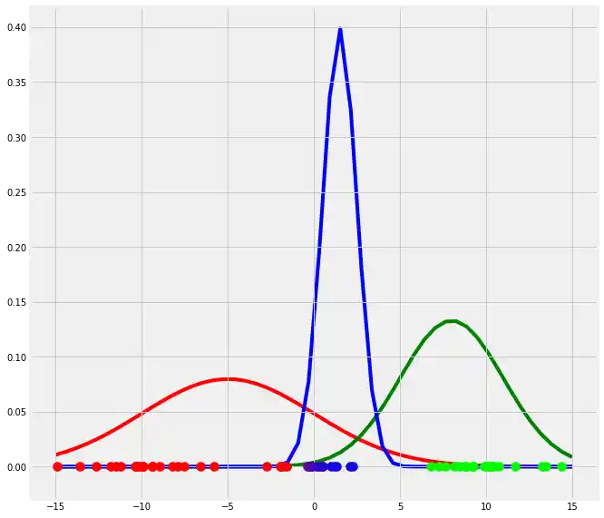
So have fitted three arbitrarily chosen gaussian models to our dataset. Therefore we have introduced a new variable which we called $r$ and in which we have stored the probability for each point $x_i$ to belong to gaussian $g$ or to cluster c, respectively. Next we have plotted the $x_i$ points and colored according to their probabilities for the three clusters. You can see that the points which have a very high probability to belong to one specific gaussian, has the color of this gaussian while the points which are between two gaussians have a color which is a mixture of the colors of the corresponding gaussians.

So in a more mathematical notation and for multidimensional cases (here the single mean value $\mu$ for the calculation of each gaussian changes to a mean vector $\boldsymbol{\mu}$ with one entry per dimension and the single variance value $\sigma^2$ per gaussian changes to a nxn covariance matrix $\boldsymbol{\Sigma}$ where n is the number of dimensions in the dataset.) the Expectation step of the EM algorithm looks like:

$\underline{E-Step}$

1. Decide how many sources/clusters (c) you want to fit to your data --> Mind that each cluster c is represented by gaussian g
2. Initialize the parameters mean $\mu_c$, covariance $\Sigma_c$, and fraction_per_class $\pi_c$ per cluster c
3. Calculate for each datapoint $x_i$ the probability $r_{ic}$ that datapoint $x_i$ belongs to cluster c with:

   $$r_{ic} = \frac{\pi_c N(\boldsymbol{x_i} \ | \ \boldsymbol{\mu_c},\boldsymbol{\Sigma_c})}{\Sigma_{k=1}^K \pi_k N(\boldsymbol{x_i \ | \ \boldsymbol{\mu_k},\boldsymbol{\Sigma_k}})}$$ where $N(\boldsymbol{x} \ | \ \boldsymbol{\mu},\boldsymbol{\Sigma})$ describes the mulitvariate Gaussian with:

   $$N(\boldsymbol{x_i},\boldsymbol{\mu_c},\boldsymbol{\Sigma_c}) \ = \ \frac{1}{(2\pi)^{\frac{n}{2}}|\Sigma_c|^{\frac{1}{2}}}exp(-\frac{1}{2}(\boldsymbol{x_i}-\boldsymbol{\mu_c})^T\boldsymbol{\Sigma_c^{-1}}(\boldsymbol{x_i}-\boldsymbol{\mu_c}))$$

   $r_{ic}$ gives us for each datapoint $x_i$ the measure of: $\frac{Probability \ that \ x_i \ belongs \ to \ class \ c}{Probability \ of \ x_i \ over \ all \ classes}$ hence if $x_i$ is very close to one gaussian g, it will get a high $r_{ic}$ value for this gaussian and relatively low values otherwise.

   So why did this help us? Well, we now know the probability for each point to belong to each gaussian.
   What can we do with this information? Well, with this information we can calculate a new mean as well as a new variance (in 1D) or covariance matrix in > 1D datasets. What will be the result of that? Well, this would change the location of each gaussian in the direction of the "real" mean and would re-shape each gaussian using a value for the variance which is closer to the "real" variance. This procedure is called the Maximization step of the EM algorithm. The Maximization step looks as follows:

   $\underline{M-Step}$

   For each cluster c: Calculate the total weight $m_c$ (loosely speaking the fraction of points allocated to cluster c) and update $\pi_c$, $\mu_c$, and $\Sigma_c$ using $r_{ic}$ with:

   $$m_c \ = \ \Sigma_i r_{ic}$$

   $$\pi_c \ = \ \frac{m_c}{m}$$

   $$\boldsymbol{\mu_c} \ = \ \frac{1}{m_c}\Sigma_i r_{ic} \boldsymbol{x_i} $$

   $$\boldsymbol{\Sigma_c} \ = \ \Sigma_i r_{ic}(\boldsymbol{x_i}-\boldsymbol{\mu_c})^T(\boldsymbol{x_i}-\boldsymbol{\mu_c})$$

   Mind that you have to use the updated means in this last formula.

   So here $m_c$ is simply the fraction of points allocated to cluster c. To understand this, assume that in our $r$ we don't have probabilities between 0 and 1 but simply 0 or 1. That is, a 1 if $x_i$ belongs to $c$ and a 0 otherwise (So each row would contain one 1 and two 0 in our example above). In this case $m_c$ would be simply the number of 1s per column, that is, the number of $x_i$ allocated to each cluster $c$. But since we have probabilities, we do not simply have ones and zeros but the principal is the same --> We sum up the probabilities $r_ic$ over all i to get $m_c$. Then $\pi_c$ is simply the fraction of points which belong to cluster c as above. We then calculate the new mean (vector) $\boldsymbol{\mu_c}$ by summing up the product of each value $x_i$ and the corresponding probability that this point belongs to cluster c ($r_{ic}$) and divide this sum by "the number of points" in c ($m_c$). Remember that if we had zeros and ones, this would be a completely normal mean calculation but since we have probabilities, we divide by the sum of these probabilities per cluster c. Also the new covariance matrix ($\boldsymbol{\Sigma_c}$) is updated by calculating the covariance matrix per class c ($\boldsymbol{\Sigma_c}$) weighted by the probability that point $x_i$ belongs to cluster c. We could also write $\boldsymbol{\Sigma_c}=m_c(\boldsymbol{x}-\boldsymbol{\mu_c})^T((\boldsymbol{x}-\boldsymbol{\mu_c}))$.
   so let's look at our plot if we do the above updates, that is run the first EM iteration .
   

import matplotlib.pyplot as plt
from matplotlib import style
style.use('fivethirtyeight')
import numpy as np
from scipy.stats import norm
np.random.seed(0)

X = np.linspace(-5,5,num=20)
X0 = X*np.random.rand(len(X))+10 # Create data cluster 1
X1 = X*np.random.rand(len(X))-10 # Create data cluster 2
X2 = X*np.random.rand(len(X)) # Create data cluster 3
X_tot = np.stack((X0,X1,X2)).flatten() # Combine the clusters to get the random datapoints from above

"""
E-Step
"""

"""Create the array r with dimensionality nxK"""
r = np.zeros((len(X_tot),3))  

"""Instantiate the random gaussians"""

gauss_1 = norm(loc=-5,scale=5) 
gauss_2 = norm(loc=8,scale=3)
gauss_3 = norm(loc=1.5,scale=1)

"""Instantiate the random mu_c"""
m = np.array([1/3,1/3,1/3]) # We expect to have three clusters 

pi = m/np.sum(m)


"""
Probability for each datapoint x_i to belong to gaussian g 
"""
for c,g,p in zip(range(3),[gauss_1,gauss_2,gauss_3],pi):
    r[:,c] = p*g.pdf(X_tot) # Write the probability that x belongs to gaussian c in column c. 
                          # Therewith we get a 60x3 array filled with the probability that each x_i belongs to one of the gaussians
"""
Normalize the probabilities such that each row of r sums to 1 and weight it by mu_c == the fraction of points belonging to 
cluster c
"""
for i in range(len(r)):
    r[i] = r[i]/(np.sum(pi)*np.sum(r,axis=1)[i])


"""M-Step"""


"""calculate m_c"""
m_c = []
for c in range(len(r[0])):
    m = np.sum(r[:,c])
    m_c.append(m) # For each cluster c, calculate the m_c and add it to the list m_c
    
"""calculate pi_c"""
pi_c = []
for m in m_c:
    pi_c.append(m/np.sum(m_c)) # For each cluster c, calculate the fraction of points pi_c which belongs to cluster c

"""calculate mu_c"""
mu_c = np.sum(X_tot.reshape(len(X_tot),1)*r,axis=0)/m_c


"""calculate var_c"""
var_c = []

for c in range(len(r[0])):
    var_c.append((1/m_c[c])*np.dot(((np.array(r[:,c]).reshape(60,1))*(X_tot.reshape(len(X_tot),1)-mu_c[c])).T,(X_tot.reshape(len(X_tot),1)-mu_c[c])))
  

    
    
"""Update the gaussians"""

gauss_1 = norm(loc=mu_c[0],scale=var_c[0]) 
gauss_2 = norm(loc=mu_c[1],scale=var_c[1])
gauss_3 = norm(loc=mu_c[2],scale=var_c[2])



"""Plot the data"""

fig = plt.figure(figsize=(10,10))
ax0 = fig.add_subplot(111)


for i in range(len(r)):
    ax0.scatter(X_tot[i],0,c=np.array([r[i][0],r[i][1],r[i][2]]),s=100) 


"""Plot the gaussians"""


for g,c in zip([gauss_1.pdf(np.sort(X_tot).reshape(60,1)),gauss_2.pdf(np.sort(X_tot).reshape(60,1)),gauss_3.pdf(np.sort(X_tot).reshape(60,1))],['r','g','b']):
    ax0.plot(np.sort(X_tot),g,c=c)

    

    
plt.show()

So as you can see the occurrence of our gaussians changed dramatically after the first EM iteration. Let's update $r$ and illustrate the coloring of the points.

"""update r"""

"""
Probability for each datapoint x_i to belong to gaussian g 
"""
# Mind that we use the new pi_c here
for c,g,p in zip(range(3),[gauss_1,gauss_2,gauss_3],pi):
    r[:,c] = p*g.pdf(X_tot) 
"""
Normalize the probabilities such that each row of r sums to 1 and weight it by mu_c == the fraction of points belonging to 
cluster c
"""
for i in range(len(r)):
    r[i] = r[i]/(np.sum(pi_c)*np.sum(r,axis=1)[i])


"""Plot the data"""

fig = plt.figure(figsize=(10,10))
ax0 = fig.add_subplot(111)



for i in range(len(r)):
    ax0.scatter(X_tot[i],0,c=np.array([r[i][0],r[i][1],r[i][2]]),s=100) # We have defined the first column as red, the second as
                                                                        # green and the third as blue

        
"""Plot the gaussians"""

for g,c in zip([gauss_1.pdf(np.sort(X_tot).reshape(60,1)),gauss_2.pdf(np.sort(X_tot).reshape(60,1)),gauss_3.pdf(np.sort(X_tot).reshape(60,1))],['r','g','b']):
    ax0.plot(np.sort(X_tot),g,c=c)
        
        
        
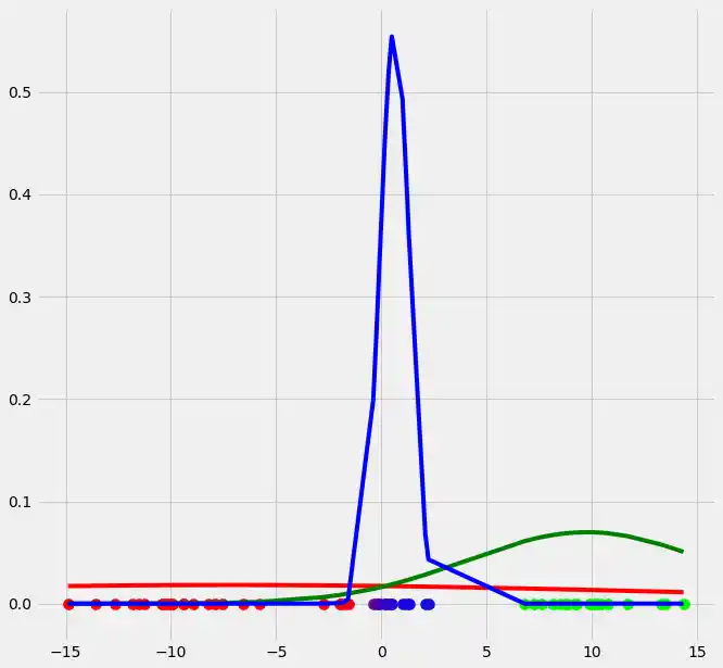
plt.show()

As you can see, the colors of the datapoints changed due to the adjustment of $r$. This is logical since also the means and the variances of the gaussians changed and therewith the allocation probabilities changed as well. Though, after this first run of our EM algorithm, the results does not look better than our initial, arbitrary starting results isn't it? Lets see what happens if we run the steps above multiple times. This is done by simply looping through the EM steps after we have done out first initializations of $\boldsymbol{\mu_c}$, $\sigma_c^2$ and $\mu_c$. We run the EM for 10 loops and plot the result in each loop. You can observe the progress for each EM loop below.

import matplotlib.pyplot as plt
from matplotlib import style
style.use('fivethirtyeight')
import numpy as np
from scipy.stats import norm
np.random.seed(0)

X = np.linspace(-5,5,num=20)
X0 = X*np.random.rand(len(X))+15 # Create data cluster 1
X1 = X*np.random.rand(len(X))-15 # Create data cluster 2
X2 = X*np.random.rand(len(X)) # Create data cluster 3
X_tot = np.stack((X0,X1,X2)).flatten() # Combine the clusters to get the random datapoints from above

class GM1D:

    def __init__(self,X,iterations):
        self.iterations = iterations
        self.X = X
        self.mu = None
        self.pi = None
        self.var = None
  

    def run(self):
        

        """
        Instantiate the random mu, pi and var
        """
        self.mu = [-8,8,5]
        self.pi = [1/3,1/3,1/3]
        self.var = [5,3,1]
        
        
        
        """
        E-Step
        """
        
        for iter in range(self.iterations):

            """Create the array r with dimensionality nxK"""
            r = np.zeros((len(X_tot),3))  

  
            """
            Probability for each datapoint x_i to belong to gaussian g 
            """
            for c,g,p in zip(range(3),[norm(loc=self.mu[0],scale=self.var[0]),
                                       norm(loc=self.mu[1],scale=self.var[1]),
                                       norm(loc=self.mu[2],scale=self.var[2])],self.pi):
                r[:,c] = p*g.pdf(X_tot) # Write the probability that x belongs to gaussian c in column c. 
                                      # Therewith we get a 60x3 array filled with the probability that each x_i belongs to one of the gaussians
            """
            Normalize the probabilities such that each row of r sums to 1 and weight it by mu_c == the fraction of points belonging to 
            cluster c
            """
            for i in range(len(r)):
                r[i] = r[i]/(np.sum(pi)*np.sum(r,axis=1)[i])


            """Plot the data"""

            fig = plt.figure(figsize=(10,10))
            ax0 = fig.add_subplot(111)


            for i in range(len(r)):
                ax0.scatter(self.X[i],0,c=np.array([r[i][0],r[i][1],r[i][2]]),s=100) 


            """Plot the gaussians"""


            for g,c in zip([norm(loc=self.mu[0],scale=self.var[0]).pdf(np.linspace(-20,20,num=60)),
                            norm(loc=self.mu[1],scale=self.var[1]).pdf(np.linspace(-20,20,num=60)),
                            norm(loc=self.mu[2],scale=self.var[2]).pdf(np.linspace(-20,20,num=60))],['r','g','b']):
                ax0.plot(np.linspace(-20,20,num=60),g,c=c)
            
            
            
            """M-Step"""
    

            """calculate m_c"""
            m_c = []
            for c in range(len(r[0])):
                m = np.sum(r[:,c])
                m_c.append(m) # For each cluster c, calculate the m_c and add it to the list m_c

            """calculate pi_c"""
            for k in range(len(m_c)):
                self.pi[k] = (m_c[k]/np.sum(m_c)) # For each cluster c, calculate the fraction of points pi_c which belongs to cluster c

            """calculate mu_c"""
            self.mu = np.sum(self.X.reshape(len(self.X),1)*r,axis=0)/m_c


            """calculate var_c"""
            var_c = []

            for c in range(len(r[0])):
                var_c.append((1/m_c[c])*np.dot(((np.array(r[:,c]).reshape(60,1))*(self.X.reshape(len(self.X),1)-self.mu[c])).T,(self.X.reshape(len(self.X),1)-self.mu[c])))



            plt.show()
    

GM1D = GM1D(X_tot,10)
GM1D.run()

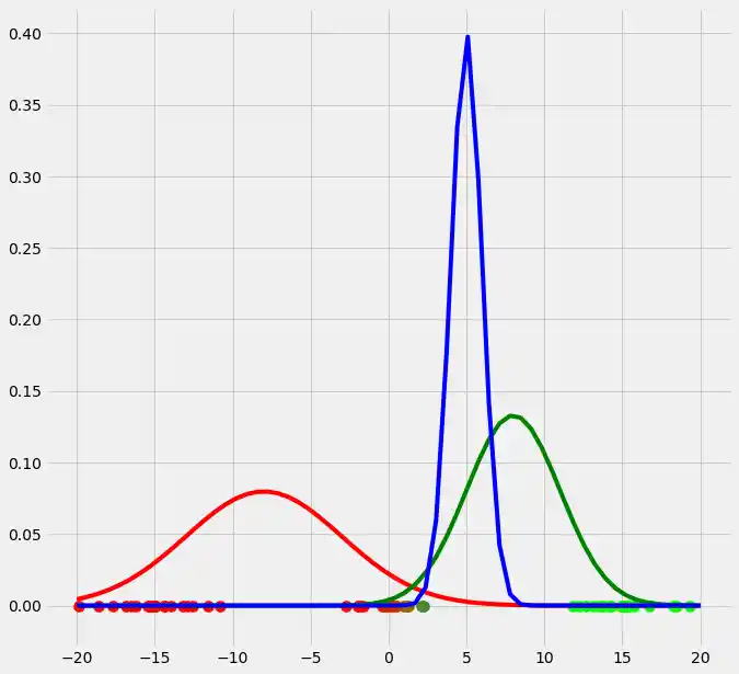
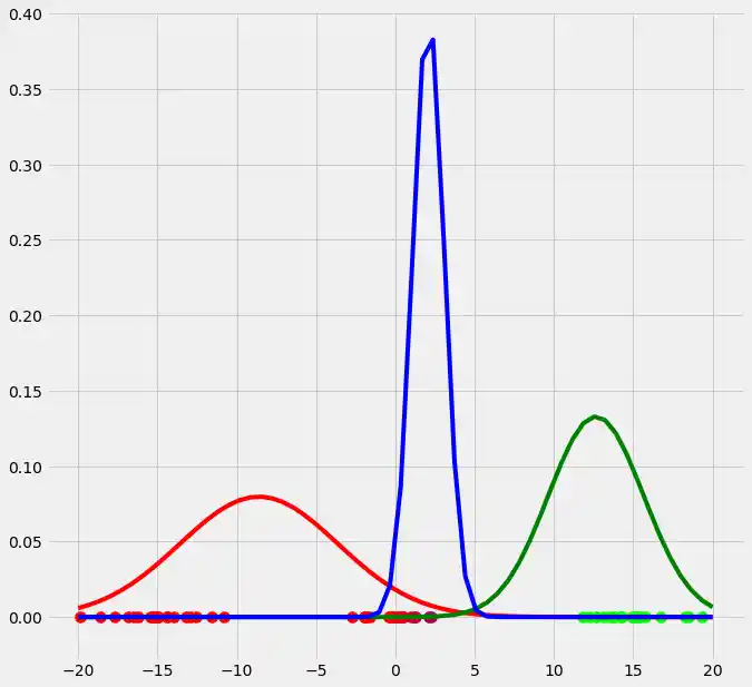
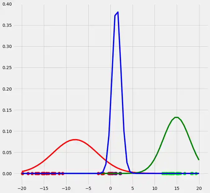
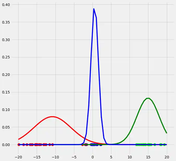
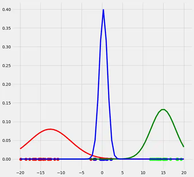
As you can see, our three randomly initialized gaussians have fitted the data. Beautiful, isn't it? The last step would now be to plot the log likelihood function to show that this function converges as the number of iterations becomes large and therewith there will be no improvement in our GMM and we can stop the algorithm to iterate. Since I have introduced this in the multidimensional case below I will skip this step here. But there isn't any magical, just compute the value of the loglikelihood as described in the pseudocode above for each iteration, save these values in a list and plot the values after the iterations. As said, I have implemented this step below and you will see how we can compute it in Python.

So we have now seen that, and how, the GMM works for the one dimensional case. But how can we accomplish this for datasets with more than one dimension? Well, it turns out that there is no reason to be afraid since once you have understand the one dimensional case, everything else is just an adaption and I still have shown in the pseudocode above, the formulas you need for the multidimensional case. So the difference to the one dimensional case is that our datasets do no longer consist of one column but have multiple columns and therewith our above $x_i$ is no longer a scalar but a vector ($\boldsymbol{x_i}$) consisting of as many elements as there are columns in the dataset. Since there are multiple columns, also the mean per class is no longer a scalar but $\mu_c$ but a vector $\boldsymbol{\mu_c}$ consisting of as many elements as there are columns in the dataset. Also, the variance is no longer a scalar for each cluster c ($\sigma^2$) but becomes a covariance matrix $\boldsymbol{\Sigma_c}$ of dimensionality nxn where n is the number of columns (dimensions) in the dataset. The calculations retain the same!

So let's derive the multi dimensional case in Python. I have added comments at all critical steps to help you to understand the code. Additionally, I have wrote the code in such a way that you can adjust how many sources (==clusters) you want to fit and how many iterations you want to run the model. By calling the EMM function with different values for number_of_sources and iterations. The actual fitting of the GMM is done in the run() function. I have also introduced a predict() function which allows us to predict the probabilities of membership for a new, unseen datapoint to belong to the fitted gaussians (clusters). So in principal, the below code is split in two parts: The run() part where we train the GMM and iteratively run through the E and M steps, and the predict() part where we predict the probability for a new datapoint. I recommend to go through the code line by line and maybe plot the result of a line with smth. like plot(result of line 44) if you are unsure what is going on -This procedure has helped the author many times-.

I have to make a final side note: I have introduced a variable called self.reg_cov. This variable is smth. we need to prevent singularity issues during the calculations of the covariance matrices. This is a mathematical problem which could arise during the calculation of the covariance matrix and hence is not critical for the understanding of the GMM itself. Though, it turns out that if we run into a singular covariance matrix, we get an error. To prevent this, we introduce the mentioned variable. For those interested in why we get a singularity matrix and what we can do against it, I will add the section "Singularity issues during the calculations of GMM" at the end of this chapter.

GMM in Python from scratch - multi dimensional case

import matplotlib.pyplot as plt
from matplotlib import style
style.use('fivethirtyeight')
from sklearn.datasets.samples_generator import make_blobs
import numpy as np
from scipy.stats import multivariate_normal


# 0. Create dataset
X,Y = make_blobs(cluster_std=1.5,random_state=20,n_samples=500,centers=3)

# Stratch dataset to get ellipsoid data
X = np.dot(X,np.random.RandomState(0).randn(2,2))


class GMM:

    def __init__(self,X,number_of_sources,iterations):
        self.iterations = iterations
        self.number_of_sources = number_of_sources
        self.X = X
        self.mu = None
        self.pi = None
        self.cov = None
        self.XY = None
        
    

    """Define a function which runs for iterations, iterations"""
    def run(self):
        self.reg_cov = 1e-6*np.identity(len(self.X[0]))
        x,y = np.meshgrid(np.sort(self.X[:,0]),np.sort(self.X[:,1]))
        self.XY = np.array([x.flatten(),y.flatten()]).T
           
                    
        """ 1. Set the initial mu, covariance and pi values"""
        self.mu = np.random.randint(min(self.X[:,0]),max(self.X[:,0]),size=(self.number_of_sources,len(self.X[0]))) # This is a nxm matrix since we assume n sources (n Gaussians) where each has m dimensions
        self.cov = np.zeros((self.number_of_sources,len(X[0]),len(X[0]))) # We need a nxmxm covariance matrix for each source since we have m features --> We create symmetric covariance matrices with ones on the digonal
        for dim in range(len(self.cov)):
            np.fill_diagonal(self.cov[dim],5)


        self.pi = np.ones(self.number_of_sources)/self.number_of_sources # Are "Fractions"
        log_likelihoods = [] # In this list we store the log likehoods per iteration and plot them in the end to check if
                             # if we have converged
            
        """Plot the initial state"""    
        fig = plt.figure(figsize=(10,10))
        ax0 = fig.add_subplot(111)
        ax0.scatter(self.X[:,0],self.X[:,1])
        ax0.set_title('Initial state')
        for m,c in zip(self.mu,self.cov):
            c += self.reg_cov
            multi_normal = multivariate_normal(mean=m,cov=c)
            ax0.contour(np.sort(self.X[:,0]),np.sort(self.X[:,1]),multi_normal.pdf(self.XY).reshape(len(self.X),len(self.X)),colors='black',alpha=0.3)
            ax0.scatter(m[0],m[1],c='grey',zorder=10,s=100)
        
        for i in range(self.iterations):               

            """E Step"""
            r_ic = np.zeros((len(self.X),len(self.cov)))

            for m,co,p,r in zip(self.mu,self.cov,self.pi,range(len(r_ic[0]))):
                co+=self.reg_cov
                mn = multivariate_normal(mean=m,cov=co)
                r_ic[:,r] = p*mn.pdf(self.X)/np.sum([pi_c*multivariate_normal(mean=mu_c,cov=cov_c).pdf(X) for pi_c,mu_c,cov_c in zip(self.pi,self.mu,self.cov+self.reg_cov)],axis=0)

            """
            The above calculation of r_ic is not that obvious why I want to quickly derive what we have done above.
            First of all the nominator:
            We calculate for each source c which is defined by m,co and p for every instance x_i, the multivariate_normal.pdf() value.
            For each loop this gives us a 100x1 matrix (This value divided by the denominator is then assigned to r_ic[:,r] which is in 
            the end a 100x3 matrix).
            Second the denominator:
            What we do here is, we calculate the multivariate_normal.pdf() for every instance x_i for every source c which is defined by
            pi_c, mu_c, and cov_c and write this into a list. This gives us a 3x100 matrix where we have 100 entrances per source c.
            Now the formula wants us to add up the pdf() values given by the 3 sources for each x_i. Hence we sum up this list over axis=0.
            This gives us then a list with 100 entries.
            What we have now is FOR EACH LOOP a list with 100 entries in the nominator and a list with 100 entries in the denominator
            where each element is the pdf per class c for each instance x_i (nominator) respectively the summed pdf's of classes c for each 
            instance x_i. Consequently we can now divide the nominator by the denominator and have as result a list with 100 elements which we
            can then assign to r_ic[:,r] --> One row r per source c. In the end after we have done this for all three sources (three loops)
            and run from r==0 to r==2 we get a matrix with dimensionallity 100x3 which is exactly what we want.
            If we check the entries of r_ic we see that there mostly one element which is much larger than the other two. This is because
            every instance x_i is much closer to one of the three gaussians (that is, much more likely to come from this gaussian) than
            it is to the other two. That is practically speaing, r_ic gives us the fraction of the probability that x_i belongs to class
            c over the probability that x_i belonges to any of the classes c (Probability that x_i occurs given the 3 Gaussians).
            """

            """M Step"""

            # Calculate the new mean vector and new covariance matrices, based on the probable membership of the single x_i to classes c --> r_ic
            self.mu = []
            self.cov = []
            self.pi = []
            log_likelihood = []

            for c in range(len(r_ic[0])):
                m_c = np.sum(r_ic[:,c],axis=0)
                mu_c = (1/m_c)*np.sum(self.X*r_ic[:,c].reshape(len(self.X),1),axis=0)
                self.mu.append(mu_c)

                # Calculate the covariance matrix per source based on the new mean
                self.cov.append(((1/m_c)*np.dot((np.array(r_ic[:,c]).reshape(len(self.X),1)*(self.X-mu_c)).T,(self.X-mu_c)))+self.reg_cov)
                # Calculate pi_new which is the "fraction of points" respectively the fraction of the probability assigned to each source 
                self.pi.append(m_c/np.sum(r_ic)) # Here np.sum(r_ic) gives as result the number of instances. This is logical since we know 
                                                # that the columns of each row of r_ic adds up to 1. Since we add up all elements, we sum up all
                                                # columns per row which gives 1 and then all rows which gives then the number of instances (rows) 
                                                # in X --> Since pi_new contains the fractions of datapoints, assigned to the sources c,
                                                # The elements in pi_new must add up to 1

            
            
            """Log likelihood"""
            log_likelihoods.append(np.log(np.sum([k*multivariate_normal(self.mu[i],self.cov[j]).pdf(X) for k,i,j in zip(self.pi,range(len(self.mu)),range(len(self.cov)))])))

            

            """
            This process of E step followed by a M step is now iterated a number of n times. In the second step for instance,
            we use the calculated pi_new, mu_new and cov_new to calculate the new r_ic which are then used in the second M step
            to calculat the mu_new2 and cov_new2 and so on....
            """

        fig2 = plt.figure(figsize=(10,10))
        ax1 = fig2.add_subplot(111) 
        ax1.set_title('Log-Likelihood')
        ax1.plot(range(0,self.iterations,1),log_likelihoods)
        #plt.show()
    
    """Predict the membership of an unseen, new datapoint"""
    def predict(self,Y):
        # PLot the point onto the fittet gaussians
        fig3 = plt.figure(figsize=(10,10))
        ax2 = fig3.add_subplot(111)
        ax2.scatter(self.X[:,0],self.X[:,1])
        for m,c in zip(self.mu,self.cov):
            multi_normal = multivariate_normal(mean=m,cov=c)
            ax2.contour(np.sort(self.X[:,0]),np.sort(self.X[:,1]),multi_normal.pdf(self.XY).reshape(len(self.X),len(self.X)),colors='black',alpha=0.3)
            ax2.scatter(m[0],m[1],c='grey',zorder=10,s=100)
            ax2.set_title('Final state')
            for y in Y:
                ax2.scatter(y[0],y[1],c='orange',zorder=10,s=100)
        prediction = []        
        for m,c in zip(self.mu,self.cov):  
            #print(c)
            prediction.append(multivariate_normal(mean=m,cov=c).pdf(Y)/np.sum([multivariate_normal(mean=mean,cov=cov).pdf(Y) for mean,cov in zip(self.mu,self.cov)]))
        #plt.show()
        return prediction
         
    
    
GMM = GMM(X,3,50)     
GMM.run()
GMM.predict([[0.5,0.5]])


 


    

[3.5799079955839772e-06, 0.00013180910068621356, 0.9998646109913182]

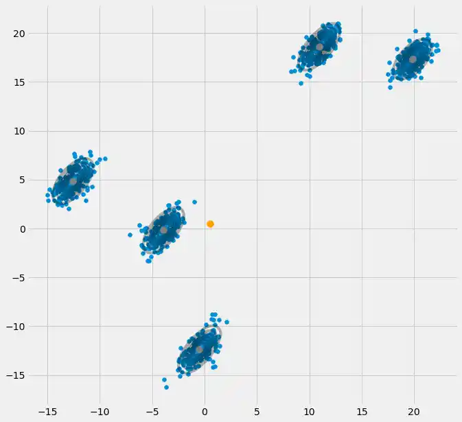
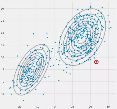
So now we have seen that we can create an arbitrary dataset, fit a GMM to this data which is first finding gaussian distributed clusters (sources) in this dataset and second allows us to predict the membership probability of an unseen datapoint to these sources.

What can we do with this model at the end of the day? Well, imagine you get a dataset like the above where someone tells you: "Hey I have a dataset and I know that there are 5 clusters. Unfortunately, I don't know which label belongs to which cluster, and hence I have a unlabeled dataset. Can you help me to find the clusters?". You can answer: "Yeah, I can by using a GMM approach!". Your opposite is delightful. A few days later the same person knocks on your door and says: "Hey I want to thank you one more time for you help. I want to let you know that I now have a new datapoint for for which I know it's target value. Can you do smth. useful with it?" you answer: "Well, I think I can. By using our created GMM model on this new datapoint, I can calculate the probability of membership of this datapoint to belong to each of the clusters. If we are lucky and our calculations return a very high probability for this datapoint for one cluster we can assume that all the datapoints belonging to this cluster have the same target value as this datapoint. Therewith, we can label all the unlabeled datapoints of this cluster (given that the clusters are tightly clustered -to be sure-). Therewith we can make a unlabeled dataset a (partly) labeled dataset and use some kind of supervised learning algorithms in the next step. Cool, isn't it?

Live Python training

Enjoying this page? We offer live Python training courses covering the content of this site.

See: Live Python courses overview

Enrol here

GMM using sklearn

So now we will create a GMM Model using the prepackaged sklearn.mixture.GaussianMixture method. As we can see, the actual set up of the algorithm, that is the instantiation as well as the calling of the fit() method does take us only one line of code. Cool isn't it?

import matplotlib.pyplot as plt
from matplotlib import style
style.use('fivethirtyeight')
from sklearn.datasets.samples_generator import make_blobs
import numpy as np
from scipy.stats import multivariate_normal
from sklearn.mixture import GaussianMixture

# 0. Create dataset
X,Y = make_blobs(cluster_std=0.5,random_state=20,n_samples=1000,centers=5)

# Stratch dataset to get ellipsoid data
X = np.dot(X,np.random.RandomState(0).randn(2,2))

x,y = np.meshgrid(np.sort(X[:,0]),np.sort(X[:,1]))
XY = np.array([x.flatten(),y.flatten()]).T

GMM = GaussianMixture(n_components=5).fit(X) # Instantiate and fit the model
print('Converged:',GMM.converged_) # Check if the model has converged
means = GMM.means_ 
covariances = GMM.covariances_


# Predict
Y = np.array([[0.5],[0.5]])
prediction = GMM.predict_proba(Y.T)
print(prediction)

# Plot   
fig = plt.figure(figsize=(10,10))
ax0 = fig.add_subplot(111)
ax0.scatter(X[:,0],X[:,1])
ax0.scatter(Y[0,:],Y[1,:],c='orange',zorder=10,s=100)
for m,c in zip(means,covariances):
    multi_normal = multivariate_normal(mean=m,cov=c)
    ax0.contour(np.sort(X[:,0]),np.sort(X[:,1]),multi_normal.pdf(XY).reshape(len(X),len(X)),colors='black',alpha=0.3)
    ax0.scatter(m[0],m[1],c='grey',zorder=10,s=100)
    
plt.show()

Converged: True
[[9.36305075e-82 1.94756664e-93 4.00098007e-33 5.02664415e-44
  1.00000000e+00]]

So as you can see, we get very nice results. Congratulations, Done!

Singularity issues during the calculations of GMM

This section will give an insight into what is happening that leads to a singular covariance matrix during the fitting of an GMM to a dataset, why this is happening, and what we can do to prevent that.

Therefore we best start by recapitulating the steps during the fitting of a Gaussian Mixture Model to a dataset.

1. Decide how many sources/clusters (c) you want to fit to your data
   
2. Initialize the parameters mean $\mu_c$, covariance $\Sigma_c$, and fraction_per_class $\pi_c$ per cluster c
   

$\underline{E-Step}$

1. Calculate for each datapoint $x_i$ the probability $r_{ic}$ that datapoint $x_i$ belongs to cluster c with:

   $$r_{ic} = \frac{\pi_c N(\boldsymbol{x_i} \ | \ \boldsymbol{\mu_c},\boldsymbol{\Sigma_c})}{\Sigma_{k=1}^K \pi_k N(\boldsymbol{x_i \ | \ \boldsymbol{\mu_k},\boldsymbol{\Sigma_k}})}$$ where $N(\boldsymbol{x} \ | \ \boldsymbol{\mu},\boldsymbol{\Sigma})$ describes the mulitvariate Gaussian with:

   $$N(\boldsymbol{x_i},\boldsymbol{\mu_c},\boldsymbol{\Sigma_c}) \ = \ \frac{1}{(2\pi)^{\frac{n}{2}}|\Sigma_c|^{\frac{1}{2}}}exp(-\frac{1}{2}(\boldsymbol{x_i}-\boldsymbol{\mu_c})^T\boldsymbol{\Sigma_c^{-1}}(\boldsymbol{x_i}-\boldsymbol{\mu_c}))$$

   $r_{ic}$ gives us for each datapoint $x_i$ the measure of: $\frac{Probability \ that \ x_i \ belongs \ to \ class \ c}{Probability \ of \ x_i \ over \ all \ classes}$ hence if $x_i$ is very close to one gaussian c, it will get a high $r_{ic}$ value for this gaussian and relatively low values otherwise.

   $\underline{M-Step}$

   For each cluster c: Calculate the total weight $m_c$ (loosely speaking the fraction of points allocated to cluster c) and update $\pi_c$, $\mu_c$, and $\Sigma_c$ using $r_{ic}$ with:

   $$m_c \ = \ \Sigma_i r_ic$$
   

   $$\pi_c \ = \ \frac{m_c}{m}$$
   

   $$\boldsymbol{\mu_c} \ = \ \frac{1}{m_c}\Sigma_i r_{ic} \boldsymbol{x_i} $$
   

   $$\boldsymbol{\Sigma_c} \ = \ \frac{1}{m_c}\Sigma_i r_{ic}(\boldsymbol{x_i}-\boldsymbol{\mu_c})^T(\boldsymbol{x_i}-\boldsymbol{\mu_c})$$
   Mind that you have to use the updated means in this last formula.

   Iteratively repeat the E and M step until the log-likelihood function of our model converges where the log likelihood is computed with:

   $$ln \ p(\boldsymbol{X} \ | \ \boldsymbol{\pi},\boldsymbol{\mu},\boldsymbol{\Sigma}) \ = \ \Sigma_{i=1}^N \ ln(\Sigma_{k=1}^K \pi_k N(\boldsymbol{x_i} \ | \ \boldsymbol{\mu_k},\boldsymbol{\Sigma_k}))$$

So now we have derived the single steps during the calculation we have to consider what it mean for a matrix to be singular. A matrix is singular if it is not invertible. A matrix is invertible if there is a matrix $X$ such that $AX = XA = I$. If this is not given, the matrix is said to be singular. That is, a matrix like:

\begin{bmatrix} 0 & 0 \\ 0 & 0 \end{bmatrix}

is not invertible and following singular. It is also plausible, that if we assume that the above matrix is matrix $A$ there could not be a matrix $X$ which gives dotted with this matrix the identity matrix $I$ (Simply take this zero matrix and dot-product it with any other 2x2 matrix and you will see that you will always get the zero matrix). But why is this a problem for us? Well, consider the formula for the multivariate normal above. There you would find $\boldsymbol{\Sigma_c^{-1}}$ which is the invertible of the covariance matrix. Since a singular matrix is not invertible, this will throw us an error during the computation.

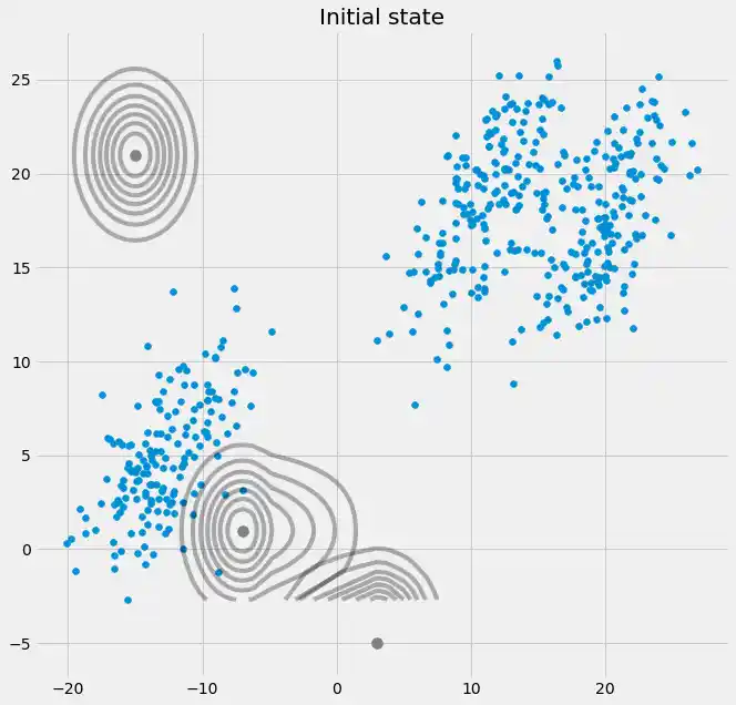
So now that we know how a singular, not invertible matrix looks like and why this is important to us during the GMM calculations, how could we ran into this issue? First of all, we get this $\boldsymbol{0}$ covariance matrix above if the Multivariate Gaussian falls into one point during the iteration between the E and M step. This could happen if we have for instance a dataset to which we want to fit 3 gaussians but which actually consists only of two classes (clusters) such that loosely speaking, two of these three gaussians catch their own cluster while the last gaussian only manages it to catch one single point on which it sits. We will see how this looks like below. But step by step: Assume you have a two dimensional dataset which consist of two clusters but you don't know that and want to fit three gaussian models to it, that is c = 3. You initialize your parameters in the E step and plot the gaussians on top of your data which looks smth. like (maybe you can see the two relatively scattered clusters on the bottom left and top right):

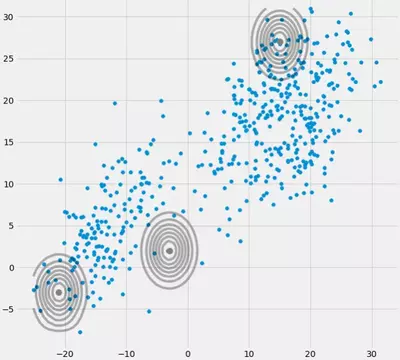
Having initialized the parameter, you iteratively do the E, T steps. During this procedure the three Gaussians are kind of wandering around and searching for their optimal place. If you observe the model parameters, that is $\mu_c$ and $\pi_c$ you will observe that they converge, that it after some number of iterations they will no longer change and therewith the corresponding Gaussian has found its place in space. In the case where you have a singularity matrix you encounter smth. like:

Where I have circled the third gaussian model with red. So you see, that this Gaussian sits on one single datapoint while the two others claim the rest. Here I have to notice that to be able to draw the figure like that I already have used covariance-regularization which is a method to prevent singularity matrices and is described below.

Ok , but now we still do not know why and how we encounter a singularity matrix. Therefore we have to look at the calculations of the $r_{ic}$ and the $cov$ during the E and M steps. If you look at the $r_{ic}$ formula again:

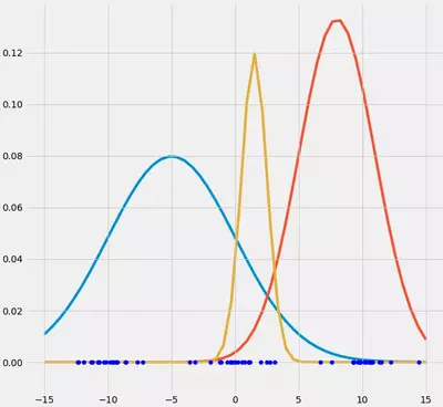
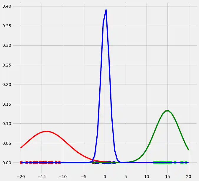
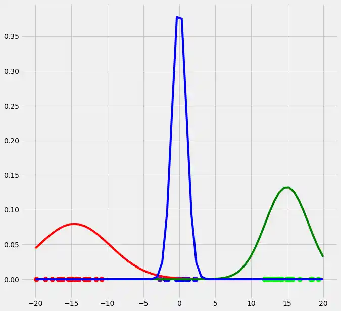
$$r_{ic} = \frac{\pi_c N(\boldsymbol{x_i} \ | \ \boldsymbol{\mu_c},\boldsymbol{\Sigma_c})}{\Sigma_{k=1}^K \pi_k N(\boldsymbol{x_i \ | \ \boldsymbol{\mu_k},\boldsymbol{\Sigma_k}})}$$ you see that there the $r_{ic}$'s would have large values if they are very likely under cluster c and low values otherwise. To make this more apparent consider the case where we have two relatively spread gaussians and one very tight gaussian and we compute the $r_{ic}$ for each datapoint $x_i$ as illustrated in the figure:

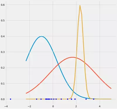
So go through the datapoints from left to right and imagine you would write down the probability for each $x_i$ that it belongs to the red, blue and yellow gaussian. What you can see is that for most of the $x_i$ the probability that it belongs to the yellow gaussian is very little. In the case above where the third gaussian sits onto one single datapoint, $r_{ic}$ is only larger than zero for this one datapoint while it is zero for every other $x_i$. (collapses onto this datapoint --> This happens if all other points are more likely part of gaussian one or two and hence this is the only point which remains for gaussian three --> The reason why this happens can be found in the interaction between the dataset itself in the initializaion of the gaussians. That is, if we had chosen other initial values for the gaussians, we would have seen another picture and the third gaussian maybe would not collapse). This is sufficient if you further and further spikes this gaussian. The $r_{ic}$ table then looks smth. like:

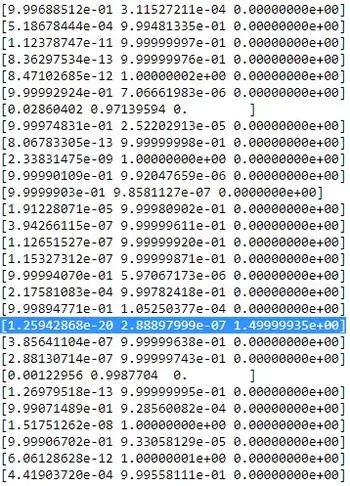
As you can see, the $r_{ic}$ of the third column, that is for the third gaussian are zero instead of this one row. If we look up which datapoint is represented here we get the datapoint: [ 23.38566343 8.07067598]. Ok, but why do we get a singularity matrix in this case? Well, and this is our last step, therefore we have to once more consider the calculation of the covariance matrix which is:

$$\boldsymbol{\Sigma_c} \ = \ \Sigma_i r_{ic}(\boldsymbol{x_i}-\boldsymbol{\mu_c})^T(\boldsymbol{x_i}-\boldsymbol{\mu_c})$$ we have seen that all $r_{ic}$ are zero instead for the one $x_i$ with [23.38566343 8.07067598]. Now the formula wants us to calculate $(\boldsymbol{x_i}-\boldsymbol{\mu_c})$. If we look at the $\boldsymbol{\mu_c}$ for this third gaussian we get [23.38566343 8.07067598]. Oh, but wait, that exactly the same as $x_i$ and that's what Bishop wrote with:"Suppose that one of the components of the mixture model, let us say the $j$ th component, has its mean $\boldsymbol{\mu_j}$ exactly equal to one of the data points so that $\boldsymbol{\mu_j} = \boldsymbol{x_n}$ for some value of n" (Bishop, 2006, p.434). So what will happen? Well, this term will be zero and hence this datapoint was the only chance for the covariance-matrix not to get zero (since this datapoint was the only one where $r_{ic}$>0), it now gets zero and looks like:

\begin{bmatrix} 0 & 0 \\ 0 & 0 \end{bmatrix}

Consequently as said above, this is a singular matrix and will lead to an error during the calculations of the multivariate gaussian. So how can we prevent such a situation. Well, we have seen that the covariance matrix is singular if it is the $\boldsymbol{0}$ matrix. Hence to prevent singularity we simply have to prevent that the covariance matrix becomes a $\boldsymbol{0}$ matrix. This is done by adding a very little value (in sklearn's GaussianMixture this value is set to 1e-6) to the digonal of the covariance matrix. There are also other ways to prevent singularity such as noticing when a gaussian collapses and setting its mean and/or covariance matrix to a new, arbitrarily high value(s). This covariance regularization is also implemented in the code below with which you get the described results. Maybe you have to run the code several times to get a singular covariance matrix since, as said. this must not happen each time but also depends on the initial set up of the gaussians.

Live Python training

Enjoying this page? We offer live Python training courses covering the content of this site.

See: Live Python courses overview

Enrol here

References

• VanderPlas,J. (2017). Python Data Science Handbook. Sebastopol: O'Reilly, pp.465
• Mitchel,T. (1997). Machine Learning. McGraw-Hill: New York, pp.191
• Bishop,P. (2006). Pattern Recognition and Machine Learning. Berlin, Heidelberg: Springer, pp.430
• https://www.youtube.com/watch?v=qMTuMa86NzU
• https://www.youtube.com/watch?v=iQoXFmbXRJA
• https://www.youtube.com/watch?v=zL_MHtT56S0
• https://www.youtube.com/watch?v=BWXd5dOkuTo

Live Python training

Enjoying this page? We offer live Python training courses covering the content of this site.

See: Live Python courses overview

Upcoming online Courses

Python Text Processing Course

Enrol here