23. A Neural Network for the Digits Dataset
By Bernd Klein. Last modified: 19 Apr 2024.
Introduction

The Python module sklear contains a dataset with handwritten digits. It is just one of many datasets which sklearn provides, as we show in our chapter Representation and Visualization of Data. In this chapter of our Machine Learning tutorial we will demonstrate how to create a neural network for the digits dataset to recognize these digits. This example is accompanying the theoretical introductions of our previous chapters to give a practical view. You will see that hardly any Python code is needed to accomplish the actual classification and recognition task.
We will first load the digits data:
from sklearn.datasets import load_digits
digits = load_digits()
We can get an overview of what is contained in the dataset with the keys method:
digits.keys()
OUTPUT:
dict_keys(['data', 'target', 'frame', 'feature_names', 'target_names', 'images', 'DESCR'])
The digits dataset contains 1797 images and each images contains 64 features, which correspond to the pixels:
n_samples, n_features = digits.data.shape
print((n_samples, n_features))
OUTPUT:
(1797, 64)
print(digits.data[0])
OUTPUT:
[ 0.  0.  5. 13.  9.  1.  0.  0.  0.  0. 13. 15. 10. 15.  5.  0.  0.  3.
 15.  2.  0. 11.  8.  0.  0.  4. 12.  0.  0.  8.  8.  0.  0.  5.  8.  0.
  0.  9.  8.  0.  0.  4. 11.  0.  1. 12.  7.  0.  0.  2. 14.  5. 10. 12.
  0.  0.  0.  0.  6. 13. 10.  0.  0.  0.]
print(digits.target)
OUTPUT:
[0 1 2 ... 8 9 8]
The data is also available at digits.images. This is the raw data of the images in the form of 8 lines and 8 columns.
With "data" an image corresponds to a one-dimensional Numpy array with the length 64, and "images" representation contains 2-dimensional numpy arrays with the shape (8, 8)
print("Shape of an item: ", digits.data[0].shape)
print("Data type of an item: ", type(digits.data[0]))
print("Shape of an item: ", digits.images[0].shape)
print("Data tpye of an item: ", type(digits.images[0]))
OUTPUT:
Shape of an item:  (64,)
Data type of an item:  <class 'numpy.ndarray'>
Shape of an item:  (8, 8)
Data tpye of an item:  <class 'numpy.ndarray'>
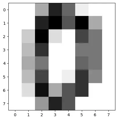
Let's visualize the data:
import matplotlib.pyplot as plt
plt.imshow(digits.images[0], cmap='binary')
plt.show()
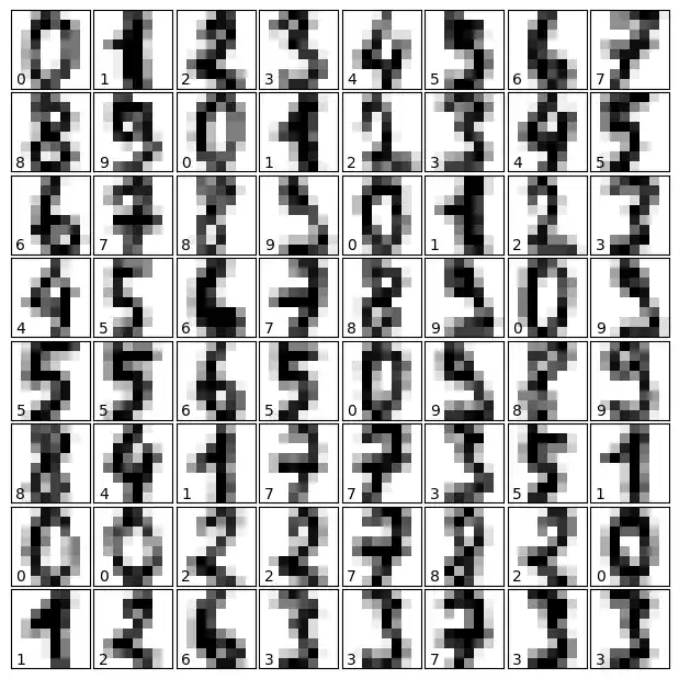
Let's visualize some more digits combined with their labels:
import matplotlib.pyplot as plt
# set up the figure
fig = plt.figure(figsize=(6, 6))  # figure size in inches
fig.subplots_adjust(left=0, right=1, bottom=0, top=1, hspace=0.05, wspace=0.05)

# plot the digits: each image is 8x8 pixels
for i in range(64):
    ax = fig.add_subplot(8, 8, i + 1, xticks=[], yticks=[])
    ax.imshow(digits.images[i], cmap=plt.cm.binary, interpolation='nearest')

    # label the image with the target value
    ax.text(0, 7, str(digits.target[i]))
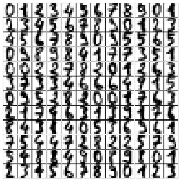
import matplotlib.pyplot as plt
# set up the figure
fig = plt.figure(figsize=(6, 6))  # figure size in inches
fig.subplots_adjust(left=0, right=1, bottom=0, top=1, hspace=0.05, wspace=0.05)

# plot the digits: each image is 8x8 pixels
for i in range(144):
    ax = fig.add_subplot(12, 12, i + 1, xticks=[], yticks=[])
    ax.imshow(digits.images[i], cmap=plt.cm.binary, interpolation='nearest')

    # label the image with the target value
    #ax.text(0, 7, str(digits.target[i]))
from sklearn.model_selection import train_test_split


res = train_test_split(digits.data, digits.target,
                       train_size=0.8,
                       test_size=0.2,
                       random_state=1)
train_data, test_data, train_labels, test_labels = res
from sklearn.neural_network import MLPClassifier

mlp = MLPClassifier(hidden_layer_sizes=(5,),
                    activation='logistic',
                    alpha=1e-4,
                    solver='sgd',
                    tol=1e-4,
                    random_state=1,
                    learning_rate_init=.3,
                    verbose=True)
mlp.fit(train_data, train_labels)
OUTPUT:
Iteration 1, loss = 2.25145782
Iteration 2, loss = 1.97730357
Iteration 3, loss = 1.66620880
Iteration 4, loss = 1.41353830
Iteration 5, loss = 1.29575643
Iteration 6, loss = 1.06663577
Iteration 7, loss = 0.95532936
Iteration 8, loss = 0.95693804
Iteration 9, loss = 1.39524681
Iteration 10, loss = 1.25724483
Iteration 11, loss = 1.18385669
Iteration 12, loss = 1.15938943
Iteration 13, loss = 1.12350490
Iteration 14, loss = 1.24327596
Iteration 15, loss = 1.12130398
Iteration 16, loss = 1.15690256
Iteration 17, loss = 1.08417899
Iteration 18, loss = 1.03437905
Training loss did not improve more than tol=0.000100 for 10 consecutive epochs. Stopping.
MLPClassifier(activation='logistic', hidden_layer_sizes=(5,),
              learning_rate_init=0.3, random_state=1, solver='sgd',
              verbose=True)MLPClassifier(activation='logistic', hidden_layer_sizes=(5,),
              learning_rate_init=0.3, random_state=1, solver='sgd',
              verbose=True)
predictions = mlp.predict(test_data)
predictions[:25] , test_labels[:25]
OUTPUT:
(array([4, 6, 0, 7, 4, 0, 6, 4, 6, 4, 3, 2, 3, 8, 4, 6, 4, 3, 7, 4, 3, 4,
        8, 6, 0]),
 array([1, 5, 0, 7, 1, 0, 6, 1, 5, 4, 9, 2, 7, 8, 4, 6, 9, 3, 7, 4, 7, 1,
        8, 6, 0]))
from sklearn.metrics import accuracy_score
accuracy_score(test_labels, predictions)
OUTPUT:
0.6305555555555555
for i in range(5, 35):
    mlp = MLPClassifier(hidden_layer_sizes=(i,),
                        activation='logistic',
                        random_state=1,
                        alpha=1e-4,
                        max_iter=10000,
                        solver='sgd',
                        tol=1e-4,
                        learning_rate_init=.3,
                        verbose=False)
    mlp.fit(train_data, train_labels)
    predictions = mlp.predict(test_data)
    acc_score = accuracy_score(test_labels, predictions)
    print(i, acc_score)
OUTPUT:
5 0.6305555555555555
6 0.6388888888888888
7 0.8777777777777778
8 0.9083333333333333
9 0.9333333333333333
10 0.9
11 0.9388888888888889
12 0.8666666666666667
13 0.9277777777777778
14 0.9777777777777777
15 0.9666666666666667
16 0.9666666666666667
17 0.9555555555555556
18 0.9583333333333334
19 0.8972222222222223
20 0.9638888888888889
21 0.9694444444444444
22 0.9722222222222222
23 0.9722222222222222
24 0.9805555555555555
25 0.9722222222222222
26 0.9722222222222222
27 0.9666666666666667
28 0.9777777777777777
29 0.9611111111111111
30 0.9694444444444444
31 0.9694444444444444
32 0.975
33 0.9694444444444444
34 0.9666666666666667
Live Python training

Enjoying this page? We offer live Python training courses covering the content of this site.
Upcoming online Courses
See our Python training courses