4. Numerical Operations on Numpy Arrays
By Bernd Klein. Last modified: 24 Mar 2022.

We have seen lots of operators in our Python tutorial. Of course, we have also seen many cases of operator overloading, e.g. "+" for the addition of numerical values and the concatenation of strings.
42 + 5
"Python is one of the best " + "or maybe the best programming language!"
We will learn in this introduction that the operator signs are overloaded in Numpy as well, so that they can be used in a "natural" way.
We can, for example, add a scalar to an ndarrays, i.e. the scalar will be added to every component. The same is possible for subtraction, division, multiplication and even for applying functions, like sine, cosine and so on, to an array.
It is also extremely easy to use all these operators on two arrays as well.
Using Scalars
Let's start with adding scalars to arrays:
import numpy as np
lst = [2,3, 7.9, 3.3, 6.9, 0.11, 10.3, 12.9]
v = np.array(lst)
v = v + 2
print(v)
OUTPUT:
[ 4. 5. 9.9 5.3 8.9 2.11 12.3 14.9 ]
Multiplication, Subtraction, Division and exponentiation are as easy as the previous addition:
print(v * 2.2)
OUTPUT:
[ 8.8 11. 21.78 11.66 19.58 4.642 27.06 32.78 ]
print(v - 1.38)
OUTPUT:
[ 2.62 3.62 8.52 3.92 7.52 0.73 10.92 13.52]
print(v ** 2)
print(v ** 1.5)
OUTPUT:
[ 16.      25.      98.01    28.09    79.21     4.4521 151.29   222.01  ]
[ 8.         11.18033989 31.14962279 12.2015163  26.55125232  3.06495204
 43.13776768 57.51477202]
We started this example with a list lst, which we turned into the array v. Do you know how to perform the above operations on a list, i.e. multiply, add, subtract and exponentiate every element of the list with a scalar?
We could use a for loop for this purpose. Let us do it for the addition without loss of generality. We will add the value 2 to every element of the list:
lst = [2,3, 7.9, 3.3, 6.9, 0.11, 10.3, 12.9]
res = []
for val in lst:
    res.append(val + 2)

print(res)
OUTPUT:
[4, 5, 9.9, 5.3, 8.9, 2.11, 12.3, 14.9]
Even though this solution works it is not the Pythonic way to do it. We will rather use a list comprehension for this purpose than the clumsy solution above. If you are not familar with this approach, you may consult our chapter on list comprehension in our Python course.
res = [ val + 2 for val in lst]
print(res)
OUTPUT:
[4, 5, 9.9, 5.3, 8.9, 2.11, 12.3, 14.9]
Even though we had already measured the time consumed by Numpy compared to "plane" Python, we will compare these two approaches as well:
v = np.random.randint(0, 100, 1000)

%timeit v + 1
OUTPUT:
869 ns ± 32.1 ns per loop (mean ± std. dev. of 7 runs, 1000000 loops each)
lst = list(v)

%timeit [ val + 2 for val in lst]
OUTPUT:
148 µs ± 8.54 µs per loop (mean ± std. dev. of 7 runs, 10000 loops each)
Live Python training

Enjoying this page? We offer live Python training courses covering the content of this site.
Arithmetic Operations with two Arrays
If we use another array instead of a scalar, the elements of both arrays will be component-wise combined:
import numpy as np

A = np.array([ [11, 12, 13], [21, 22, 23], [31, 32, 33] ])
B = np.ones((3,3))

print("Adding to arrays: ")
print(A + B)

print("\nMultiplying two arrays: ")
print(A * (B + 1))
OUTPUT:
Adding to arrays:
[[12. 13. 14.]
 [22. 23. 24.]
 [32. 33. 34.]]

Multiplying two arrays:
[[22. 24. 26.]
 [42. 44. 46.]
 [62. 64. 66.]]
"A * B" in the previous example shouldn't be mistaken for matrix multiplication. The elements are solely component-wise multiplied.
Matrix Multiplication:
For this purpose, we can use the dot product. Using the previous arrays, we can calculate the matrix multiplication:
np.dot(A, B)
OUTPUT:
array([[36., 36., 36.],
       [66., 66., 66.],
       [96., 96., 96.]])
Definition of the dot Product
The dot product is defined like this:
dot(a, b, out=None)
For 2-D arrays the dot product is equivalent to matrix multiplication. For 1-D arrays it is the same as the inner product of vectors (without complex conjugation). For N dimensions it is a sum product over the last axis of 'a' and the second-to-last of 'b'::
| Parameter | Meaning |
|---|---|
| a | array or array like argument |
| b | array or array like argument |
| out | 'out' is an optional parameter, which must have the exact kind of what would be returned, if it was not used. This is a performance feature. Therefore, if these conditions are not met, an exception is raised, instead of attempting to be flexible. |
The function dot returns the dot product of 'a' and 'b'. If 'a' and 'b' are both scalars or both 1-D arrays then a scalar is returned; otherwise an array will returned.
It will raise a ValueError, if the shape of the last dimension of 'a' is not the same size as the shape of the second-to-last dimension of 'b', i.e. a.shape[-1] == b.shape[-2]
Examples of Using the dot Product
We will begin with the cases in which both arguments are scalars or one-dimensional array:
print(np.dot(3, 4))
x = np.array([3])
y = np.array([4])
print(x.ndim)
print(np.dot(x, y))

x = np.array([3, -2])
y = np.array([-4, 1])
print(np.dot(x, y))
OUTPUT:
12
1
12
-14
Let's go to the two-dimensional use case:
A = np.array([ [1, 2, 3],
               [3, 2, 1] ])
B = np.array([ [2, 3, 4, -2],
               [1, -1, 2, 3],
               [1, 2, 3, 0] ])

# es muss gelten:
print(A.shape[-1] == B.shape[-2], A.shape[1])
print(np.dot(A, B))
OUTPUT:
True 3
[[ 7  7 17  4]
 [ 9  9 19  0]]
We can learn from the previous example that the number of columns of the first two-dimension array have to be the same as the number of the lines of the second two-dimensional array.
The dot Product in the 3-dimensional Case
It's getting really vexing, if we use 3-dimensional arrays as the arguments of dot.
We will use two symmetrical three-dimensional arrays in the first example:
import numpy as np
X = np.array( [[[3, 1, 2],
                [4, 2, 2],
                [2, 4, 1]],

               [[3, 2, 2],
                [4, 4, 3],
                [4, 1, 1]],

               [[2, 2, 1],
                [3, 1, 3],
                [3, 2, 3]]])

Y = np.array( [[[2, 3, 1],
                [2, 2, 4],
                [3, 4, 4]],

               [[1, 4, 1],
                [4, 1, 2],
                [4, 1, 2]],

               [[1, 2, 3],
                [4, 1, 1],
                [3, 1, 4]]])


R = np.dot(X, Y)

print("The shapes:")
print(X.shape)
print(Y.shape)
print(R.shape)

print("\nThe Result R:")
print(R)
OUTPUT:
The shapes:
(3, 3, 3)
(3, 3, 3)
(3, 3, 3, 3)

The Result R:
[[[[14 19 15]
   [15 15  9]
   [13  9 18]]

  [[18 24 20]
   [20 20 12]
   [18 12 22]]

  [[15 18 22]
   [22 13 12]
   [21  9 14]]]


 [[[16 21 19]
   [19 16 11]
   [17 10 19]]

  [[25 32 32]
   [32 23 18]
   [29 15 28]]

  [[13 18 12]
   [12 18  8]
   [11 10 17]]]


 [[[11 14 14]
   [14 11  8]
   [13  7 12]]

  [[17 23 19]
   [19 16 11]
   [16 10 22]]

  [[19 25 23]
   [23 17 13]
   [20 11 23]]]]
To demonstrate how the dot product in the three-dimensional case works, we will use different arrays with non-symmetrical shapes in the following example:
import numpy as np
X = np.array(
    [[[3, 1, 2],
      [4, 2, 2]],

     [[-1, 0, 1],
      [1, -1, -2]],

     [[3, 2, 2],
      [4, 4, 3]],

     [[2, 2, 1],
      [3, 1, 3]]])

Y = np.array(
    [[[2, 3, 1, 2, 1],
      [2, 2, 2, 0, 0],
      [3, 4, 0, 1, -1]],

     [[1, 4, 3, 2, 2],
      [4, 1, 1, 4, -3],
      [4, 1, 0, 3, 0]]])


R = np.dot(X, Y)


print("X.shape: ", X.shape, "   X.ndim: ", X.ndim)
print("Y.shape: ", Y.shape, "   Y.ndim: ", Y.ndim)
print("R.shape: ",     R.shape, "R.ndim: ", R.ndim)


print("\nThe result array R:\n")
print(R)
OUTPUT:
X.shape:  (4, 2, 3)    X.ndim:  3
Y.shape:  (2, 3, 5)    Y.ndim:  3
R.shape:  (4, 2, 2, 5) R.ndim:  4

The result array R:

[[[[ 14  19   5   8   1]
   [ 15  15  10  16   3]]

  [[ 18  24   8  10   2]
   [ 20  20  14  22   2]]]


 [[[  1   1  -1  -1  -2]
   [  3  -3  -3   1  -2]]

  [[ -6  -7  -1   0   3]
   [-11   1   2  -8   5]]]


 [[[ 16  21   7   8   1]
   [ 19  16  11  20   0]]

  [[ 25  32  12  11   1]
   [ 32  23  16  33  -4]]]


 [[[ 11  14   6   5   1]
   [ 14  11   8  15  -2]]

  [[ 17  23   5   9   0]
   [ 19  16  10  19   3]]]]
Let's have a look at the following sum products:
i = 0
for j in range(X.shape[1]):
    for k in range(Y.shape[0]):
        for m in range(Y.shape[2]):
            fmt = "    sum(X[{}, {}, :] * Y[{}, :, {}] :  {}"
            arguments = (i, j, k, m, sum(X[i, j, :] * Y[k, :, m]))
            print(fmt.format(*arguments))
OUTPUT:
    sum(X[0, 0, :] * Y[0, :, 0] :  14
    sum(X[0, 0, :] * Y[0, :, 1] :  19
    sum(X[0, 0, :] * Y[0, :, 2] :  5
    sum(X[0, 0, :] * Y[0, :, 3] :  8
    sum(X[0, 0, :] * Y[0, :, 4] :  1
    sum(X[0, 0, :] * Y[1, :, 0] :  15
    sum(X[0, 0, :] * Y[1, :, 1] :  15
    sum(X[0, 0, :] * Y[1, :, 2] :  10
    sum(X[0, 0, :] * Y[1, :, 3] :  16
    sum(X[0, 0, :] * Y[1, :, 4] :  3
    sum(X[0, 1, :] * Y[0, :, 0] :  18
    sum(X[0, 1, :] * Y[0, :, 1] :  24
    sum(X[0, 1, :] * Y[0, :, 2] :  8
    sum(X[0, 1, :] * Y[0, :, 3] :  10
    sum(X[0, 1, :] * Y[0, :, 4] :  2
    sum(X[0, 1, :] * Y[1, :, 0] :  20
    sum(X[0, 1, :] * Y[1, :, 1] :  20
    sum(X[0, 1, :] * Y[1, :, 2] :  14
    sum(X[0, 1, :] * Y[1, :, 3] :  22
    sum(X[0, 1, :] * Y[1, :, 4] :  2
Hopefully, you have noticed that we have created the elements of R[0], one ofter the other.
print(R[0])
OUTPUT:
[[[14 19  5  8  1]
  [15 15 10 16  3]]

 [[18 24  8 10  2]
  [20 20 14 22  2]]]
This means that we could have created the array R by applying the sum products in the way above. To "prove" this, we will create an array R2 by using the sum product, which is equal to R in the following example:
R2 = np.zeros(R.shape, dtype=np.int8)

for i in range(X.shape[0]):
    for j in range(X.shape[1]):
        for k in range(Y.shape[0]):
            for m in range(Y.shape[2]):
                R2[i, j, k, m] = sum(X[i, j, :] * Y[k, :, m])


print( np.array_equal(R, R2) )
OUTPUT:
True
Live Python training
Enjoying this page? We offer live Python training courses covering the content of this site.
Upcoming online Courses
Matrices vs. Two-Dimensional Arrays
Some may have taken two-dimensional arrays of Numpy as matrices. This is principially all right, because they behave in most aspects like our mathematical idea of a matrix. We even saw that we can perform matrix multiplication on them. Yet, there is a subtle difference. There are "real" matrices in Numpy. They are a subset of the two-dimensional arrays. We can turn a two-dimensional array into a matrix by applying the "mat" function. The main difference shows, if you multiply two two-dimensional arrays or two matrices. We get real matrix multiplication by multiplying two matrices, but the two-dimensional arrays will be only multiplied component-wise:
import numpy as np

A = np.array([ [1, 2, 3], [2, 2, 2], [3, 3, 3] ])
B = np.array([ [3, 2, 1], [1, 2, 3], [-1, -2, -3] ])

R = A * B
print(R)
OUTPUT:
[[ 3  4  3]
 [ 2  4  6]
 [-3 -6 -9]]
MA = np.mat(A)
MB = np.mat(B)

R = MA * MB
print(R)
OUTPUT:
[[ 2  0 -2]
 [ 6  4  2]
 [ 9  6  3]]
Comparison Operators
We are used to comparison operators from Python, when we apply them to integers, floats or strings for example. We use them to test for True or False. If we compare two arrays, we don't get a simple True or False as a return value. The comparisons are performed elementswise. This means that we get a Boolean array as a return value:
import numpy as np

A = np.array([ [11, 12, 13], [21, 22, 23], [31, 32, 33] ])
B = np.array([ [11, 102, 13], [201, 22, 203], [31, 32, 303] ])

A == B
OUTPUT:
array([[ True, False,  True],
       [False,  True, False],
       [ True,  True, False]])
It is possible to compare complete arrays for equality as well. We use array_equal for this purpose. array_equal returns True if two arrays have the same shape and elements, otherwise False will be returned.
print(np.array_equal(A, B))
print(np.array_equal(A, A))
OUTPUT:
False
True
Live Python training
Enjoying this page? We offer live Python training courses covering the content of this site.
Logical Operators
We can also apply the logical 'or' and the logical 'and' to arrays elementwise. We can use the functions 'logical_or' and 'logical_and' to this purpose.
a = np.array([ [True, True], [False, False]])
b = np.array([ [True, False], [True, False]])

print(np.logical_or(a, b))
print(np.logical_and(a, b))
OUTPUT:
[[ True  True]
 [ True False]]
[[ True False]
 [False False]]
Applying Operators on Arrays with Different Shapes
So far we have covered two different cases with basic operators like "+" or "*":
- an operator applied to an array and a scalar
- an operator applied to two arrays of the same shape
We will see in the following that we can also apply operators on arrays, if they have different shapes. Yet, it works only under certain conditions.
Live Python training
Enjoying this page? We offer live Python training courses covering the content of this site.
Broadcasting
Numpy provides a powerful mechanism, called Broadcasting, which allows to perform arithmetic operations on arrays of different shapes. This means that we have a smaller array and a larger array, and we transform or apply the smaller array multiple times to perform some operation on the larger array. In other words: Under certain conditions, the smaller array is "broadcasted" in a way that it has the same shape as the larger array.
With the aid of broadcasting we can avoid loops in our Python program. The looping occurs implicitly in the Numpy implementations, i.e. in C. We also avoid creating unnecessary copies of our data.
We demonstrate the operating principle of broadcasting in three simple and descriptive examples.
First example of broadcasting:
import numpy as np

A = np.array([ [11, 12, 13], [21, 22, 23], [31, 32, 33] ])
B = np.array([1, 2, 3])

print("Multiplication with broadcasting: ")
print(A * B)
print("... and now addition with broadcasting: ")
print(A + B)
OUTPUT:
Multiplication with broadcasting:
[[11 24 39]
 [21 44 69]
 [31 64 99]]
... and now addition with broadcasting:
[[12 14 16]
 [22 24 26]
 [32 34 36]]
The following diagram illustrates the way of working of broadcasting:
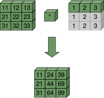
B is treated as if it were construed like this:
B = np.array([[1, 2, 3],] * 3)
print(B)
OUTPUT:
[[1 2 3]
 [1 2 3]
 [1 2 3]]
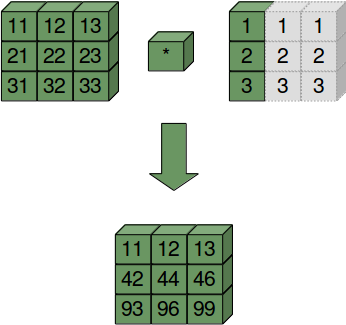
Second Example:
For this example, we need to know how to turn a row vector into a column vector:
B = np.array([1, 2, 3])
B[:, np.newaxis]
OUTPUT:
array([[1],
       [2],
       [3]])
Now we are capable of doing the multipliplication using broadcasting:
A * B[:, np.newaxis]
OUTPUT:
array([[11, 12, 13],
       [42, 44, 46],
       [93, 96, 99]])
B is treated as if it were construed like this:
np.array([[1, 2, 3],] * 3).transpose()
OUTPUT:
array([[1, 1, 1],
       [2, 2, 2],
       [3, 3, 3]])
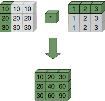
Third Example:
A = np.array([10, 20, 30])
B = np.array([1, 2, 3])
A[:, np.newaxis]
OUTPUT:
array([[10],
       [20],
       [30]])
A[:, np.newaxis] * B
OUTPUT:
array([[10, 20, 30],
       [20, 40, 60],
       [30, 60, 90]])
Another Way to Do it
Doing it without broadcasting:
import numpy as np

A = np.array([ [11, 12, 13], [21, 22, 23], [31, 32, 33] ])

B = np.array([1, 2, 3])

B = B[np.newaxis, :]
B = np.concatenate((B, B, B))

print("Multiplication: ")
print(A * B)
print("... and now addition again: ")
print(A + B)
OUTPUT:
Multiplication:
[[11 24 39]
 [21 44 69]
 [31 64 99]]
... and now addition again:
[[12 14 16]
 [22 24 26]
 [32 34 36]]
Using 'tile':
import numpy as np

A = np.array([ [11, 12, 13], [21, 22, 23], [31, 32, 33] ])

B = np.tile(np.array([1, 2, 3]), (3, 1))

print(B)

print("Multiplication: ")
print(A * B)
print("... and now addition again: ")
print(A + B)
OUTPUT:
[[1 2 3]
 [1 2 3]
 [1 2 3]]
Multiplication:
[[11 24 39]
 [21 44 69]
 [31 64 99]]
... and now addition again:
[[12 14 16]
 [22 24 26]
 [32 34 36]]
Live Python training
Enjoying this page? We offer live Python training courses covering the content of this site.
Distance Matrix
In mathematics, computer science and especially graph theory, a distance matrix is a matrix or a two-dimensional array, which contains the distances between the elements of a set, pairwise taken. The size of this two-dimensional array in n x n, if the set consists of n elements.
A practical example of a distance matrix is a distance matrix between geographic locations, in our example Eurpean cities:
cities = ["Barcelona", "Berlin", "Brussels", "Bucharest",
          "Budapest", "Copenhagen", "Dublin", "Hamburg", "Istanbul",
          "Kiev", "London", "Madrid", "Milan", "Moscow", "Munich",
          "Paris", "Prague", "Rome", "Saint Petersburg",
          "Stockholm", "Vienna", "Warsaw"]

dist2barcelona = [0,  1498, 1063, 1968,
                  1498, 1758, 1469, 1472, 2230,
                  2391, 1138, 505, 725, 3007, 1055,
                  833, 1354, 857, 2813,
                  2277, 1347, 1862]

dists =  np.array(dist2barcelona[:12])
print(dists)
print(np.abs(dists - dists[:, np.newaxis]))
OUTPUT:
[   0 1498 1063 1968 1498 1758 1469 1472 2230 2391 1138  505]
[[   0 1498 1063 1968 1498 1758 1469 1472 2230 2391 1138  505]
 [1498    0  435  470    0  260   29   26  732  893  360  993]
 [1063  435    0  905  435  695  406  409 1167 1328   75  558]
 [1968  470  905    0  470  210  499  496  262  423  830 1463]
 [1498    0  435  470    0  260   29   26  732  893  360  993]
 [1758  260  695  210  260    0  289  286  472  633  620 1253]
 [1469   29  406  499   29  289    0    3  761  922  331  964]
 [1472   26  409  496   26  286    3    0  758  919  334  967]
 [2230  732 1167  262  732  472  761  758    0  161 1092 1725]
 [2391  893 1328  423  893  633  922  919  161    0 1253 1886]
 [1138  360   75  830  360  620  331  334 1092 1253    0  633]
 [ 505  993  558 1463  993 1253  964  967 1725 1886  633    0]]
3-Dimensional Broadcasting
A = np.array([ [[3, 4, 7], [5, 0, -1] , [2, 1, 5]],
      [[1, 0, -1], [8, 2, 4], [5, 2, 1]],
      [[2, 1, 3], [1, 9, 4], [5, -2, 4]]])

B = np.array([ [[3, 4, 7], [1, 0, -1], [1, 2, 3]] ])

B * A
OUTPUT:
array([[[ 9, 16, 49],
        [ 5,  0,  1],
        [ 2,  2, 15]],

       [[ 3,  0, -7],
        [ 8,  0, -4],
        [ 5,  4,  3]],

       [[ 6,  4, 21],
        [ 1,  0, -4],
        [ 5, -4, 12]]])
We will use the following transformations in our chapter on Images Manipulation and Processing:
B = np.array([1, 2, 3])

B = B[np.newaxis, :]
print(B.shape)
B = np.concatenate((B, B, B)).transpose()
print(B.shape)
B = B[:, np.newaxis]
print(B.shape)
print(B)

print(A * B)
OUTPUT:
(1, 3)
(3, 3)
(3, 1, 3)
[[[1 1 1]]

 [[2 2 2]]

 [[3 3 3]]]
[[[ 3  4  7]
  [ 5  0 -1]
  [ 2  1  5]]

 [[ 2  0 -2]
  [16  4  8]
  [10  4  2]]

 [[ 6  3  9]
  [ 3 27 12]
  [15 -6 12]]]
Live Python training
Enjoying this page? We offer live Python training courses covering the content of this site.
Upcoming online Courses