24. Naive Bayes Classification with Python
By Bernd Klein. Last modified: 19 Apr 2024.
Definition

In machine learning, a Bayes classifier is a simple probabilistic classifier, which is based on applying Bayes' theorem. The feature model used by a naive Bayes classifier makes strong independence assumptions. This means that the existence of a particular feature of a class is independent or unrelated to the existence of every other feature.
Definition of independent events:
Two events E and F are independent, if both E and F have positive probability and if P(E|F) = P(E) and P(F|E) = P(F)
As we have stated in our definition, the Naive Bayes Classifier is based on the Bayes' theorem. The Bayes theorem is based on the conditional probability, which we will define now:
Live Python training

Enjoying this page? We offer live Python training courses covering the content of this site.
Conditional Probability
$P(A|B)$ stands for "the conditional probability of A given B", or "the probability of A under the condition B", i.e. the probability of some event A under the assumption that the event B took place. When in a random experiment the event B is known to have occurred, the possible outcomes of the experiment are reduced to B, and hence the probability of the occurrence of A is changed from the unconditional probability into the conditional probability given B. The Joint probability is the probability of two events in conjunction. That is, it is the probability of both events together. There are three notations for the joint probability of A and B. It can be written as
- $P(A ∩ B)$
- $P(AB)$ or
- $P(A,B)$
The conditional probability is defined by
Examples for Conditional Probability
German Swiss Speaker
There are about 8.4 million people living in Switzerland. About 64 % of them speak German. There are about 7500 million people on earth.
If some aliens randomly beam up an earthling, what are the chances that he is a German speaking Swiss?
We have the events
S: being Swiss
GS: German Speaking
The probability for a randomly chosen person to be Swiss:
If we know that somebody is Swiss, the probability of speaking German is 0.64. This corresponds to the conditional probability
So the probability of the earthling being Swiss and speaking German, can be calculated by the formula:
inserting the values from above gives us:
and
So our aliens end up with a chance of 0.07168 % of getting a German speaking Swiss person.
False Positives and False Negatives
A medical research lab proposes a screening to test a large group of people for a disease. An argument against such screenings is the problem of false positive screening results.
Suppose 0,1% of the group suffer from the disease, and the rest is well:
and
The following is true for a screening test:
If you have the disease, the test will be positive 99% of the time, and if you don't have it, the test will be negative 99% of the time:
P("test positive" | "well") = 1 %
and
P("test negative" | "well") = 99 %.
Finally, suppose that when the test is applied to a person having the disease, there is a 1% chance of a false negative result (and 99% chance of getting a true positive result), i.e.
P("test negative" | "sick") = 1 %
and
P("test positive" | "sick") = 99 %
| Sick |
Healthy |
Totals |
|
| Test
result positive |
99 |
999 |
1098 |
| Test
result negative |
1 |
98901 |
98902 |
| Totals |
100 |
99900 |
100000 |
There are 999 False Positives and 1 False Negative.
Problem:
In many cases even medical professionals assume that "if you have this sickness, the test will be positive in 99 % of the time and if you don't have it, the test will be negative 99 % of the time. Out of the 1098 cases that report positive results only 99 (9 %) cases are correct and 999 cases are false positives (91 %), i.e. if a person gets a positive test result, the probability that he or she actually has the disease is just about 9 %. P("sick" | "test positive") = 99 / 1098 = 9.02 %
Live Python training
Enjoying this page? We offer live Python training courses covering the content of this site.
Upcoming online Courses
Bayes' Theorem
We calculated the conditional probability $P(GS | S)$, which was the probability that a person speaks German, if he or she is known to be Swiss. To calculate this we used the following equation:
What about calculating the probability $P(S | GS)$, i.e. the probability that somebody is Swiss under the assumption that the person speeks German?
The equation looks like this:
Let's isolate on both equations $P(GS, S)$:
As the left sides are equal, the right sides have to be equal as well:
This equation can be transformed into:
The result corresponts to Bayes' theorem
To solve our problem, - i.e. the probability that a person is Swiss, if we know that he or she speaks German - all we have to do is calculate the right side. We know already from our previous exercise that
and
The number of German native speakers in the world corresponds to 101 millions, so we know that
Finally, we can calculate $P(S | GS)$ by substituting the values in our equation:
There are about 8.4 million people living in Switzerland. About 64 % of them speak German. There are about 7500 million people on earth.
If the some aliens randomly beam up an earthling, what are the chances that he is a German speaking Swiss?
We have the events
$S$: being Swiss $GS$: German Speaking
$P(A|B)$ is the conditional probability of $A$, given $B$ (posterior probability), $P(B)$ is the prior probability of $B$ and $P(A)$ the prior probability of $A$. $P(B|A)$ is the conditional probability of $B$ given $A$, called the likely-hood.
An advantage of the naive Bayes classifier is that it requires only a small amount of training data to estimate the parameters necessary for classification. Because independent variables are assumed, only the variances of the variables for each class need to be determined and not the entire covariance matrix.
Naive Bayes Classifier
Live Python training
Enjoying this page? We offer live Python training courses covering the content of this site.
Introductory Exercise

Let's set out on a journey by train to create our first very simple Naive Bayes Classifier. Let us assume we are in the city of Hamburg and we want to travel to Munich. We will have to change trains in Frankfurt am Main. We know from previous train journeys that our train from Hamburg might be delayed and the we will not catch our connecting train in Frankfurt. The probability that we will not be in time for our connecting train depends on how high our possible delay will be. The connecting train will not wait for more than five minutes. Sometimes the other train is delayed as well.
The following lists 'in_time' (the train from Hamburg arrived in time to catch the connecting train to Munich) and 'too_late' (connecting train is missed) are data showing the situation over some weeks. The first component of each tuple shows the minutes the train was late and the second component shows the number of time this occurred.
# the tuples consist of (delay time of train1, number of times)


# tuples are (minutes, number of times)
in_time = [(0, 22), (1, 19), (2, 17), (3, 18),
           (4, 16), (5, 15), (6, 9), (7, 7),
           (8, 4), (9, 3), (10, 3), (11, 2)]
too_late = [(6, 6), (7, 9), (8, 12), (9, 17),
            (10, 18), (11, 15), (12,16), (13, 7),
            (14, 8), (15, 5)]
%matplotlib inline

import matplotlib.pyplot as plt

X, Y = zip(*in_time)

X2, Y2 = zip(*too_late)

bar_width = 0.9
plt.bar(X, Y, bar_width,  color="blue", alpha=0.75, label="in time")
bar_width = 0.8
plt.bar(X2, Y2, bar_width,  color="red", alpha=0.75, label="too late")
plt.legend(loc='upper right')
plt.show()
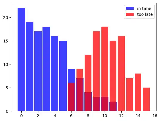
From this data we can deduce that the probability of catching the connecting train if we are one minute late is 1, because we had 19 successful cases experienced and no misses, i.e. there is no tuple with 1 as the first component in 'too_late'.
We will denote the event "train arrived in time to catch the connecting train" with $S$ (success) and the 'unlucky' event "train arrived too late to catch the connecting train" with $M$ (miss)
We can now define the probability "catching the train given that we are 1 minute late" formally:
We used the fact that the tuple $(1, 19)$ is in 'in_time' and there is no tuple with the first component 1 in 'too_late'
It's getting critical for catching the connecting train to Munich, if we are 6 minutes late. Yet, the chances are still 60 %:
Accordingly, the probability for missing the train knowing that we are 6 minutes late is:
We can write a 'classifier' function, which will give the probability for catching the connecting train:
in_time_dict = dict(in_time)
too_late_dict = dict(too_late)

def catch_the_train(min):
    s = in_time_dict.get(min, 0)
    if s == 0:
        return 0
    else:
        m = too_late_dict.get(min, 0)
        return s / (s + m)

for minutes in range(-1, 13):
    print(minutes, catch_the_train(minutes))
OUTPUT:
-1 0
0 1.0
1 1.0
2 1.0
3 1.0
4 1.0
5 1.0
6 0.6
7 0.4375
8 0.25
9 0.15
10 0.14285714285714285
11 0.11764705882352941
12 0
A NaiveBayes Classifier
The following class NaiveBayesClassifier encapsulates the training and prediction logic of a Naive Bayes Classifier, making it easy to train on data and make predictions on new samples. It's worth noting that this implementation assumes categorical features, as it calculates probabilities based on the occurrence of discrete feature values.
from collections import defaultdict
import numpy as np

class NaiveBayesClassifier:
    def __init__(self):
        self.class_probs = {}
        self.feature_probs = {}

    def fit(self, X, y):
        """  This method takes input data `X` (features) and `y`
        (labels) and calculates the probabilities needed for classification.
        It first calculates the probabilities of each class occurring in the
        dataset (`class_probs`).
        Then, it calculates for each class the probabilities of each feature
        given the class (`feature_probs`).
        It uses Laplace smoothing to handle cases where a feature value is
        unseen in the training data."""

        # Calculate class probabilities
        class_counts = defaultdict(int)
        for label in y:
            class_counts[label] += 1
        total_samples = len(y)
        for label, count in class_counts.items():
            self.class_probs[label] = count / total_samples

        # Calculate feature probabilities
        self.feature_probs = {}
        for label in self.class_probs:
            #create a boolean array (label_indices) indicating which samples
            # in the dataset have the current class label:
            label_indices = (y == label)
            # This selects the samples from the input dataset X that belong
            # to the current class:
            label_X = X[label_indices]
            feature_probs = {}
            for feature in range(X.shape[1]):
                feature_counts = defaultdict(int)
                for sample in label_X:
                    feature_val = sample[feature]
                    feature_counts[feature_val] += 1
                total_samples_label = len(label_X)
                feature_probs[feature] = {val: count / total_samples_label for val, count in feature_counts.items()}


                feature_probs[feature] = {val: (count + 1) / (total_samples_label + len(feature_counts))  # Laplace smoothing
                                                 for val, count in feature_counts.items()}
            self.feature_probs[label] = feature_probs

    def _calculate_probability(self, x, feature, label):
        """ This method calculates the probability of a given feature
        value occurring given a class label."""
        if x in self.feature_probs[label][feature]:
            return self.feature_probs[label][feature][x]
        else:
            return 1e-6  # Smoothing for unseen feature values

    def _predict_sample(self, x):
        """  This method predicts the label of a single sample by
        calculating the probability of each class given the sample's
        features and selecting the class with the highest
        probability."""
        max_prob = -1
        best_label = None
        for label, class_prob in self.class_probs.items():
            prob = class_prob
            for feature, value in enumerate(x):
                prob *= self._calculate_probability(value, feature, label)
            if prob > max_prob:
                max_prob = prob
                best_label = label
        return best_label

    def predict(self, X):
        """ This method takes input data `X` and predicts the labels for each sample using
        the `_predict_sample` method. """
        return [self._predict_sample(sample) for sample in X]
The _predict_sample method calculates the probability of each class label given a single sample's features and selects the class label with the highest probability. The formula for calculating the probability of a class label $ C_k $ given a sample $ \mathbf{x} $ is based on Bayes' theorem and the assumption of feature independence (hence, "naive" Bayes):
where:
- $ P(C_k | \mathbf{x}) $ is the posterior probability of class $ C_k $ given the sample $ \mathbf{x} $.
- $ P(\mathbf{x} | C_k) $ is the likelihood of observing the sample $ \mathbf{x} $ given class $ C_k $. This is calculated by multiplying the probabilities of each feature value given class $ C_k $.
- $ P(C_k) $ is the prior probability of class $ C_k $, which is stored in
self.class_probs. - $ P(\mathbf{x}) $ is the probability of observing the sample $ \mathbf{x} $. Since this is a constant for all classes, it is not needed for selecting the most probable class and can be omitted.
The _predict_sample method calculates the posterior probability $ P(C_k | \mathbf{x}) $ for each class $ C_k $ using the above formula and selects the class with the highest posterior probability as the predicted class label for the sample.
We will use and test our NaiveBayesClassifier with the following data:
# Data
data = [
    ["Strawberry", "Red", "Smooth", "Sweet", "Desserts", "Fruit"],
    ["Celery", "Green", "Crisp", "Mild", "Salads", "Vegetable"],
    ["Pineapple", "Yellow", "Rough", "Sweet", "Snacks", "Fruit"],
    ["Spinach", "Green", "Tender", "Mild", "Salads", "Vegetable"],
    ["Blueberry", "Blue", "Smooth", "Sweet", "Baking", "Fruit"],
    ["Cucumber", "Green", "Crisp", "Mild", "Salads", "Vegetable"],
    ["Watermelon", "Red", "Juicy", "Sweet", "Snacks", "Fruit"],
    ["Carrot", "Orange", "Crunchy", "Sweet", "Salads", "Vegetable"],
    ["Grapes", "Purple", "Juicy", "Sweet", "Snacks", "Fruit"],
    ["Bell Pepper", "Red", "Crisp", "Mild", "Cooking", "Vegetable"],
    ["Kiwi", "Brown", "Fuzzy", "Tart", "Snacks", "Fruit"],
    ["Lettuce", "Green", "Tender", "Mild", "Salads", "Vegetable"],
    ["Mango", "Orange", "Smooth", "Sweet", "Desserts", "Fruit"],
    ["Potato", "Brown", "Starchy", "Mild", "Cooking", "Vegetable"],
    ["Apple", "Red", "Crunchy", "Sweet", "Snacks", "Fruit"],
    ["Onion", "White", "Firm", "Pungent", "Cooking", "Vegetable"],
    ["Orange", "Orange", "Smooth", "Sweet", "Snacks", "Fruit"],
    ["Garlic", "White", "Firm", "Pungent", "Cooking", "Vegetable"],
    ["Peach", "Orange", "Smooth", "Sweet", "Desserts", "Fruit"],
    ["Broccoli", "Green", "Tender", "Mild", "Cooking", "Vegetable"],
    ["Cherry", "Red", "Juicy", "Sweet", "Snacks", "Fruit"],
    ["Peas", "Green", "Soft", "Sweet", "Cooking", "Vegetable"],
    ["Pear", "Green", "Juicy", "Sweet", "Snacks", "Fruit"],
    ["Cabbage", "Green", "Crisp", "Mild", "Cooking", "Vegetable"],
    ["Grapefruit", "Pink", "Juicy", "Tart", "Snacks", "Fruit"],
    ["Asparagus", "Green", "Tender", "Mild", "Cooking", "Vegetable"]
]
The following code prepares data for machine learning by converting it into a Numpy array, separating features and labels, encoding categorical features into numerical values, and partitioning the dataset into training and test sets.
# Convert data to a numpy array
data = np.array(data)

# Split features and labels
X = data[:, :-1]  # Features
y = data[:, -1]   # Labels

# Encode categorical features into numerical values
# Encode categorical features into numerical values using a single LabelEncoder
label_encoder = LabelEncoder()
X_encoded = np.array([label_encoder.fit_transform(sample) for sample in X])


# Split data into training and test sets
X_train = X_encoded[:20]
y_train = y[:20]
X_test = X_encoded[20:]
y_test = y[20:]
This code trains a Naive Bayes classifier (nb_classifier) on the provided training data
(X_train and y_train). Once trained, it predicts labels for the test data (X_test)
using the predict method, storing the predictions in y_pred. This process enables
evaluating the classifier's performance on unseen data.
# Train the classifier
nb_classifier = NaiveBayesClassifier()
nb_classifier.fit(X_train, y_train)

# Predict on the test data
y_pred = nb_classifier.predict(X_test)

y_pred
OUTPUT:
['Fruit', 'Fruit', 'Fruit', 'Vegetable', 'Fruit', 'Vegetable']
This code calculates the accuracy of the predictions made by the classifier. It iterates over each pair of predicted and true labels in the test dataset (y_pred and y_test, respectively), counting the number of correct predictions. Then, it divides the number of correct predictions by the total number of predictions to compute the accuracy. Finally, it prints out the calculated accuracy.
# Calculate accuracy
correct_predictions = sum(1 for pred, true in zip(y_pred, y_test) if pred == true)
total_predictions = len(y_test)
accuracy = correct_predictions / total_predictions
print("Accuracy:", accuracy)
OUTPUT:
Accuracy: 0.8333333333333334
Live Python training
Enjoying this page? We offer live Python training courses covering the content of this site.
The Underlying Theory
Our classifier from the previous example is based on the Bayes theorem:
where
-
$P(c_j | d)$ is the probability of instance d being in class c_j, it is the result we want to calculate with our classifier
-
$P(d | c_j)$ is the probability of generating the instance d, if the class $c_j$ is given
-
$P(c_j)$ is the probability for the occurrence of class $c_j$ We didn't use it in our classifiers, because both classes in our example have been equally likely.
- P(d) is the probability for the occurrence of an instance d It's not needed in the calculation, because it is the same for all classes.
We had used only one feature in our previous examples, i.e. the 'height' or the name.
It's possible to define a Bayes Classifier with multiple features, e.g. $d = (d_1, d_2, ..., d_n)$
We get the following formula:
$\frac{1}{P(d)}$ is only depending on the values of $d_1, d_2, ... d_n$. This means that it is a constant as the values of the feature variables are known.
Live Python training
Enjoying this page? We offer live Python training courses covering the content of this site.
Upcoming online Courses